Azimuth

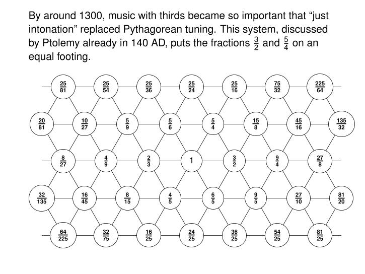
In this series I’ve been explaining 12-tone scales in just intonation—or more precisely, ‘5-limit’ just intonation, where all the frequency ratios are integer powers of the primes 2, 3 and 5. There are various choices involved in building such a scale. A lot of famous mathematicians have tried their hand at it. Kepler, Descartes, Mersenne, Newton, Mercator, and Euler are among them. They didn’t agree on the best scale: they came up with different scales.

Newton did his work on this in college when he was 22. This was 1665, the year he later fled Trinity College to avoid the Great Plague, went to the countryside, invented calculus, began thinking about gravity, and discovered that a prism can recombine colors of light to make white light.

Given this, I can’t resist classifying all possible scales of this sort. Today we’ll see that by a certain precise definition, there are 174,240 such scales! It will take a bit of combinatorics to work this out. Among this large collection of scales we will also find smaller sets of scales with nice properties. But I still don’t know why those mathematicians chose the scales they did.

In studying this, and indeed in all my work on just intonation, I was greatly helped by this wonderful paper:

• Daniel Muzzulini, Isaac Newton’s microtonal approach to just intonation, Empirical Musicology Review 15 (2021), 223–248.

It’s full of interesting diagrams:

Anyway, let’s get going!

In Part 2 of this series, I examined the choices involved in building a just intonation scale. I described a general recipe for building such scales. These leads to 2 × 4 × 2 = 16 different scales, based on how you make the choices here:

tonic		1
minor 2nd		16/15
major 2nd		10/9 or 9/8
minor 3rd		6/5
major 3rd		5/4
perfect 4th		4/3
tritone		25/18 or 45/32 or 64/45 or 36/25
perfect 5th		3/2
minor 6th		8/5
major 6th		5/3
minor 7th		16/9 or 9/5
major 7th		15/8
octave		2

Newton’s scale is one of these 16. Marin Mersenne had created the same scale in 1636, but Newton probably didn’t know this. In fact I studied this scale in Part 4, where I claimed that it’s the most popular just intonation scale of all! It’s hard to be sure of that—but I certainly think it’s the nicest one.

Here it is:

The intervals between the notes come in 3 different sizes, which we will discuss soon. In Part 4, I explained some reasons this scale is nice. For example, the intervals here are nearly palindromic! The first interval is the same as the last, and so on—except right near the middle of the scale, the ‘tritone’, where this symmetry is impossible because it would force to be a rational number.

In Part 4, I also considered another less popular scale among the 16 generated by my recipe:

In this one the intervals come in 4 different sizes! Let’s make up abbreviations for them. In order of increasing size, they are:

• c: the lesser chromatic semitone, with frequency ratio 25/24 = 1.041666…

• C: the greater chromatic semitone, with frequency ratio 135/128 = 1.0546875.

• d: the diatonic semitone, with a frequency ratio of 16/15 = 1.0666…

• D: the large diatonic semitone, with frequency ratio 27/25 = 1.08.

With this notation, Newton’s scale is

I’ll say this scale has type (2,3,7,0) since it has 2 c’s, 3 C’s, 7 d’s and 0 D’s. The less popular scale I mentioned is

This scale has type (3,2,6,1). Arguably this scale is worse, because the large diatonic semitone is quite large compared to all the rest.

Muzzulini also describes some other just intonation scales. Here’s one that Nicolas Mercator created around 1660—not the Mercator with the map, the one who discovered the power series for the logarithm:

This is striking because it has two large diatonic semitones: it’s of type (4,1,5,2).

Here’s one that the music theorist William Holder wrote down in 1694:

This has three diatonic semitones—the most possible! It’s of type (5,0,4,3).

Leonhard Euler came up with this scale in 1739:

This has type (3,2,6,1).

It would be interesting to find out, if possible, why various authors chose the scales they did. Did they scan the universe of possibilities and try to pick a scale that was optimal in some way—or did they did they just make one up? Answering this would require some historical investigation.

All these ruminations led me to some questions about enumerating and classifying scales, which I included as puzzles in Part 4. Now let me finally answer them!

Puzzle 1. As we’ve seen, the most popular 12-tone just intonation scale is of type (2,3,7,0). That is, it has 2 lesser chromatic semitones, 3 greater chromatic semitones, 7 diatonic semitones, and no large diatonic semitones. By permuting these semitones we can get many other scales. How many different scales can we get this way?

Answer. We have a 12-element set and we’re asking: in how many ways can we partition it into a 2-element set, a 3-element set and a 7-element set? This is the kind of question that multinomial coefficients were designed to answer. The answer is

  █

Puzzle 2. Our second, less popular 12-tone just intonation scale is of type (3,2,6,1): it has 3 lesser chromatic semitones, 2 greater chromatic semitones, 6 diatonic semitones and 1 large diatonic semitone. How many other scales can we get by permuting these semitones?

Answer. By the same reasoning, we have

such scales.   █

These puzzles were warmups for a bigger question:

Puzzle 3. How many 12-tone scales are there where the spacing between each pair of successive notes is either a lesser chromatic semitone, a greater chromatic semitone, a diatonic semitone, or a large diatonic semitone?

Answer. The only types of scales allowed are quadruples of nonnegative integers where

or equivalently,

The four numbers

span the 3-dimensional rational vector space with basis so they must obey one linear relation with integer coefficients (and others following from this one). This relation is

This says cD = Cd: the lesser chromatic semitone followed by the large diatonic semitone takes you up to a frequency 9/8 higher, just like the greater chromatic semitone followed by the diatonic semitone.

This means that if a type is allowed, so is if Furthermore, it means this move (and its inverse) can take you from any allowed type to all other allowed types.

So, let’s start with the type where the number of large diatonic semitones, is as small as possible. This is our friend

(2,3,7,0)

We can get all other allowed types by repeatedly adding 1 to the first and last component of this vector and subtracting 1 from the other components. Thus, these are all the allowed types:

(2,3,7,0)
(3,2,6,1)
(4,1,5,2)
(5,0,4,3)

We can now use the methods of Puzzles 1 and 2 to count the scales of each type. We get:

= 7,920 scales of type (2,3,7,0).

= 55,440 scales of type (3,2,6,1).

= 83,160 scales of type (4,1,5,2).

= 27,720 scales of type (5,0,4,3).

So, we get a total of

7,920 + 55,440 + 83,160 + 27,720 = 174,240 scales.   █

This is a ridiculously large number of scales! But of course, not all are equally good. Let’s impose some extra constraints.

The whole point of just intonation was to make the third equal to 5/4, and we also want to keep the fourth at 4/3 and the fifth at 3/2, as we had in Pythagorean tuning. When it comes to the second, either 10/9 or 9/8 are considered acceptable in just intonation. I like 9/8 a bit better, so let’s do this:

Puzzle 4. How many 12-tone scales are there where the spacing between each pair of successive notes is either a lesser chromatic semitone, a greater chromatic semitone, a diatonic semitone, a large diatonic semitone, and:

• the second is 9/8
• the third is 5/4
• the fourth is 4/3
• the fifth is 3/2?

Answer. With these constraints there are 1,600 allowed scales. The idea is this:

• There are 4 ways to go from 1 up to 9/8 in two semitones, since only Cd, dC, cD and Dc multiply to 9/8.

• There are 2 ways to go from 9/8 up to 5/4 in two semitones, since only cd and dc multiply to 10/9.

• There is 1 way to go from 5/4 up to 4/3, since d is 16/15.

• There are 4 ways to go from 4/3 up to 3/2, since only Cd, dC, cD and Dc multiply to 9/8.

• There are 500 ways to go from 3/2 to 2 in five steps. Here we need to count ordered quintuples of c, C, d and D that multiply to 4/3. I did this with a computer.

So, we get 4 × 2 × 1 × 4 × 500 = 1,600 scales of this sort.   █

All these scales have the second being the greater major second, 9/8. But you might prefer the lesser major second, 10/9. So let’s think about that:

Puzzle 5. What about the same question as before, but where we constrain the second to be 10/9 instead of 9/8?

Answer. Again there are 1600 scales. In Puzzle 4 our scales went up from 1 to 9/8 by choosing two semitones that multiply to 9/8, and then from 9/8 to 5/4 by choosing two that multiply to 10/9. Now the only difference is that we’re going things in the other order: we’re going up from 1 to 10/9 by choosing two semitones that multiply to 10/9, and then from 10/9 to 5/4 by choosing two that multiply to 9/8. So the overall count is the same as before.   █

Since they differ only by switching some semitones, the 1,600 scales with a greater major second have the same distribution of types as the 1,600 with a lesser major second. Using a computer, I calculated that in each case there are

• 160 of type (2,3,7,0)
• 560 of type (3,2,6,1)
• 640 of type (4,1,5,2)
• 240 of type (5,0,4,3).

How can we pick out a smaller number of ‘better’ scales? We’ve imposed a lot of constraints on the tones from the first to the fifth, but none on the tones above that. To impose constraints on the higher tones, we can demand that our scale be palindromic, except that we can’t require that the interval from the fourth to the tritone equals the interval from the tritone to the fifth, because is irrational. So, I’ll call scales with the following properties nearly palindromic:

• the interval from 1 to ♭2 equals that from 7 to 8
• the interval from ♭2 to 2 equals that from ♭7 to 7
• the interval from 2 to ♭3 equals that from 6 to ♭7
• the interval from ♭3 to 3 equals that from ♭6 to 6
• the interval from 3 to 4 equals that from 5 to ♭6.

Puzzle 6. How many nearly palindromic 12-tone scales are there where the spacing between each pair of successive notes is either a lesser chromatic semitone, a greater chromatic semitone, a diatonic semitone, a large diatonic semitone, and:

• the second is 9/8
• the third is 5/4
• the fourth is 4/3?

Answer. There are 32 scales with these properties. First note that the above properties force other facts:

• the fifth is 3/4 × 2 = 3/2
• the minor sixth is 4/5 × 2 = 8/5
• the minor seventh is 8/9 × 2 = 16/9.

Thus, we have the following choices:

• There are 4 ways to go from 1 up to 9/8 in two semitones, since only Cd, dC, cD and Dc multiply to 9/8.

• There are 2 ways to go from 9/8 up to 5/4 in two semitones, since only cd and dc multiply to 10/9.

• There is 1 way to go from 5/4 up to 4/3, since d is 16/15.

• There are 4 ways to go from 4/3 up to 3/2, since only Cd, dC, cD and Dc multiply to 9/8.

and from then on, our choices are forced by the nearly palindromic nature of the scale.

There are thus a total of

4 × 2 × 1 × 4 = 32

choices.   █

These 32 scales come in two kinds:

• the 16 scales discussed in Part 4, where the minor second is the diatonic semitone, d = 16/15

• 16 others, where the minor second is the greater chromatic semitone, C = 135/128.

Newton’s scale is of the first kind.

All 32 of these scales use the greater major second. A similar story holds with the lesser major second.

Puzzle 7. How many nearly palindromic 12-tone scales are there where the spacing between each pair of successive notes is either a lesser chromatic semitone, a greater chromatic semitone, a diatonic semitone, a large diatonic semitone, and:

• the second is 10/9
• the third is 5/4
• the fourth is 4/3?

Answer. By the symmetry we used to answer Puzzle 5, this question has the same answer as Puzzle 6: there are again 32 choices.   █

These 32 scales again come in two kinds:

• 16 scales where the interval from the second to the minor third is the diatonic semitone, d = 16/15

• 16 others where the interval from the second to the minor third is the greater chromatic semitone, C = 135/128.

If you’ve made it this far, congratulations! I was lured in by how many famous mathematicians had studied this subject, and I wanted to join the fun.

---

For more on Pythagorean tuning, read this series:

• Pythagorean tuning.

For more on just intonation, read these:

• Part 1: The history of just intonation. Just intonation versus Pythagorean tuning. The syntonic comma.

• Part 2: Just intonation from the Tonnetz. The four possible tritones in just intonation. The small and large just whole tones. Ptolemy’s intense diatonic scale, and its major triads.

• Part 3: Curling up a parallelogram in the Tonnetz to get just intonation. The frequency ratios of the four possible tritones: the syntonic comma, the lesser and greater diesis, and the diaschisma.

• Part 4: Choices involved in just intonation. Two symmetrical 13-tone scales, and two 12-tone scales obtained from these by removing the diminished fifth. The four kinds of half-tone that appear in these scales: the diatonic, large diatonic, lesser chromatic and greater chromatic semitones.

• Part 5: Frequency ratios between the four possible tritones in just intonation, and how they are related to frequency ratios between the four kinds of half-tone. The syntonic comma, lesser and greater diesis, diaschisma, and the relations they obey.

• Part 6: Classifying all 174,240 12-tone scales where the intervals between successive notes are always diatonic, large diatonic, lesser chromatic and greater chromatic semitones. The scales of Isaac Newton, Nicolas Mercator, William Holder and Leonhard Euler.

For more on quarter-comma meantone tuning, read this series:

• Quarter-comma meantone.

For more on well-tempered scales, read this series:

• Well temperaments.

For more on equal temperament, read this series:

• Equal temperament.

I’m giving a talk on the math of tuning systems at Claremont McKenna College on January 30th at 11 am. If you’re around, please come! You can read my slides here:

• The mathematics of tuning systems.

But my slides don’t contain most of what I’ll write here… the stuff I’ll say out loud in my talk.

If you look at a piano keyboard you’ll see groups of 2 black notes alternating with groups of 3. So the pattern repeats after 5 black notes, but if you count you’ll see there are also 7 white notes in this repetitive pattern. So: the pattern repeats each 12 notes.

Some people who never play the piano claim it would be easier if had all white keys, or simply white alternating with black. But in fact the pattern makes it easier to keep track of where you are – and it’s not arbitrary, it’s musically significant.

For one thing white notes give a 7-note scale all their own. Most very simple songs use only this scale! The black notes also form a useful scale. And the white and black notes together form a 12-tone scale.

Starting at any note and going up 12 notes, we reach a note whose frequency is almost exactly double the one we started with. Other spacings correspond to other frequency ratios.

I don’t want to overwhelm you with numbers. So I’m only showing you a few of the simplest and most important ratios. These are really worth remembering.

We give the notes letter names. This goes back at least to Boethius, the guy famous for writing The Consolations of Philosophy before he was tortured and killed at the order of Theodoric the Great. (Yeah, “Great”.) Boethius was a counselor to Theodoric, but he really would have done better to stay out of politics – he was quite good at math and music theory.

Boethius may be the reason the lowest note on the piano is called A. We now repeat the names of the white notes as shown in the picture: seven white notes A,B,C,D,E,F,G and then it repeats.

So the scale used to start at A, using only white notes. But due to the irregular spacing of white notes, a scale of all white notes sounds different depending on where you start. Starting at A gives you the ‘minor scale’, which sounds kinda sad. Now we often start at C, since that gives us the scale most people like best: the ‘major’ scale.

(Good musicians start wherever they want, and get different sounds that way. But ‘C major’ is like the vanilla ice cream of scales—now. It wasn’t always this way.)

From the late 1100s to about 1600 people called pitches that lie outside 7-tone system ‘musica ficta’: ‘false’ or ‘fictitious’ notes. But gradually these notes—the black keys on the piano when you’re playing in C major—became more accepted.

To keep things simple for mathematicians, I’ll usually denote these with the ‘flat’ symbol, ♭. For example, G♭ is the black note one down from the white note G.

(Musicians really need both flats and sharps, and they’d also call G♭ something else: F♯. I’ll actually need both G♭ and F♯ at some points in this talk!)

Since starting the scale with the letter C takes a little practice, I’ll do it a different way that mathematicians may like better. I’ll start with 1 and count up. Musicians put little hats on these numbers, and I’ll do that.

For example, we’ll call the fifth white note up the scale the ‘fifth’ and write it as

Now for the math of tuning systems!

The big question is: how do we choose the frequency of each note? This is literally how many times per second the air vibrates, when we play that note.

Since 1850, by far the most common method for tuning keyboards has been ’12-tone equal temperament’. Here we divide each octave into 12 equal parts.

What do I mean by this, exactly? I mean that each note on the piano produces a sound that vibrates faster than the note directly below it by a factor of the 12th root of 2.

But we can contemplate ‘N-tone equal temperament’ for N = 1, 2, 3, …. – and some people do use these other tuning systems!

Here’s a picture of the most popular modern tuning system: 12-tone equal temperament. As we march around clockwise, each note has a frequency of times the note directly before it.

When we go all the way around the circle, we’ve gone up an octave. That is, we’ve reached a frequency that’s twice the one we started with.

But a note that’s an octave higher sounds ‘the same, only higher’. So in a funny way we’re back where we started.

But now for a big question: why do we use a scale with 12 notes?

To start answering, notice that we actually use three scales: one with 5 notes (the black keys), one with 7 (the white keys) and one with 12 (all the keys).

As mathematicians we can detect a highly nonobvious pattern here.

What’s so good about scales with 5, 7 or 12 notes?

A crucial clue seems to be the ‘fifth’. If you go up to the fifth white note here, its frequency is about 3/2 times the first. This is one of the simplest fractions, and it sounds incredibly simple and pure. So it’s important. It’s a dominant force in western music.

We can make a chart to see how close an approximation to the fraction 3/2 we get in a scale with N equally spaced notes.

N = 5 does better than any scale with fewer notes!

N = 7 does better than any scale with fewer notes!

N = 12 does better than any scale with fewer notes! And it does much better. To beat it, we have to go all the way up to N = 29—and even that is only slightly better.

Here’s a chart of how close we can get to a frequency ratio of 3/2 using N-tone equal temperament.

See how great 12-tone equal temperament is?

There are also some neat patterns. See the stripes of even numbers and stripes of odd numbers? That’s not a coincidence. For more charts like this, and much more cool stuff along these lines, go here.

Here’s the ‘star of fifths’ in 12-tone equal temperament!

12-tone equal temperament is most popular tuning system since maybe 1810, or definitely by 1850. But it’s mathematically the most boring of the tuning systems that have dominated Western music since the Middle Ages. Now let’s go back much earlier, to Pythagorean tuning.

When you chop the octave into 12 equal parts, the frequency ratios of all your notes are irrational numbers… except when you go up or down some number of octaves.

The Pythagoreans disliked irrational numbers. People even say they drowned Hippasus at sea after he proved that the square root of 2 is irrational! That’s just a myth, but it illustrates how people connected Pythagoras to a love of rational numbers. In Pythagorean tuning, people wanted a lot of frequency ratios of 3/2.

In equal temperament, where we chop the octave into 12 equal parts, when we start at any note and go up 7 of these parts (a so-called ‘fifth’), we reach a note that vibrates about 1.4981 times as fast. That’s close enough to 3/2 for most ears. But it’s not the Pythagorean ideal!

As we’ll see, seeking the Pythagorean ideal causes trouble. It will unleash the devil in music.

Start at some note and keep multiplying the frequency by 3/2, like a good Pythagorean. After doing this 12 times, you reach a note that’s close to 7 octaves higher. But not exactly, since the 12th power of 3/2 is

129.746338

which is a bit more than

2⁷ = 128

The ratio of these two is called the ‘Pythagorean comma’:

p = (3/2)¹² / 2⁷ = 3¹² / 2¹⁹ ≈ 1.0136

This is like an unavoidable lump in the carpet when you use Pythagorean tuning.

It’s good to stick the lump in your carpet under your couch. And it’s good to stick the Pythagorean comma near the so-called ‘tritone’—a very dissonant note that you’d tend to avoid in medieval music. This note is halfway around the circle of fifths.

In Pythagorean tuning, going 6 steps clockwise around the circle of fifths doesn’t give you the same note as going 6 steps counterclockwise! We call one of them ♭5 and the other ♯4.

Their frequency ratio is the Pythagorean comma!

In equal temperament, the tritone is exactly halfway up the octave: 6 notes up. Since going up an octave doubles the frequency, going up a tritone multiplies the frequency by √2. It’s no coincidence that this is the irrational number that got Hippasus in trouble.

In Pythagorean tuning, going 6 steps up the scale doesn’t match jumping up an octave and then going 6 steps down. We call one of them ♭5 and the other ♯4. They’re both decent approximations to √2, built from powers of 2 and 3.

Their frequency ratio is the Pythagorean comma!

The tritone is sometimes called ‘diabolus in musica’: the devil in music. Some say this interval was actually banned by the Catholic church! But that’s another myth.

It could have gotten its name because it sounds so dissonant—but mathematically, the ‘devil’ here is that the square root of 2 is irrational. If we’re trying to use only numbers built from powers of 2 and 3, we have to arbitrarily choose one to approximate √2.

In Pythagorean tuning we can choose either

1024/729 ≈ 1.4047

called the sharped fourth, ♯4, or

729/512 ≈ 1.4238

called the flatted fifth, ♭5, to be our tritone. In this chart I’ve chosen the ♭5.

No matter which you choose, one fifth in the circle of fifths will be noticeably smaller than the rest. It’s called the ‘wolf fifth’ because it howls like a wolf.

You can hear a wolf fifth here:

If you’re playing medieval music, you can easily avoid the wolf fifth: just don’t play one of the two fifths that contains the tritone!

A more practical problem concerns the ‘third’: the third white note in the scale. Ideally this vibrates 5/4 as fast as the first. But in Pythagorean tuning it vibrates 81/64 times as fast. That’s annoyingly high!

Sure, 81/64 is a rational number. But it’s not the really simple rational number our ears are hoping for when we hear a third.

Indeed, Pythagorean tuning punishes the ear with some very complicated fractions. The first, fourth, fifth and octave are great. But the rest of the notes are not. There’s no way that 243/128 sounds better than an irrational number!

In the 1300s, when thirds were becoming more important in music, theorists embraced a beautiful solution to this problem, called ‘just intonation’. Now let’s talk about that.

It’s an amazing fact that in western composed music, harmony became important only around 1200 AD, when Perotin expanded the brand new use of two-part harmony to four-part harmony.

This put pressure on musicians to use a new tuning system—or rather, to revive an old tuning system. It’s often called ‘just intonation’ (though experts will find that vague). We can get using a cool trick, though I doubt this is how it was originally discovered.

First, draw a hexagonal grid of notes. Put a note with frequency 1 in the middle. Label the other notes by saying that moving one step to the right multiplies the frequency of your note by 3/2, while going up and to the right multiplies it by 5/4.

Next, cut out a portion of the grid to use for our scale. We use this particular parallelogram—you’ll soon see what’s so great about it.

Now, multiply each number in our parallelogram by whatever power of 2 it takes to get a number between 1 and 2.

We do this because we want frequencies that lie within an octave, to be notes in a scale. Remember: if 1 is the note we started with, 2 is the note an octave up.

Now we want to curl up our parallelogram to get a torus. If we do this, gluing together opposite edges, there will be exactly 12 numbers on our torus—just right for a scale! This is a remarkable coincidence.

There’s a problem: the numbers at the corners are not all equal. But they’re pretty close! And they’re close to √2: the frequency of the tritone, the ‘devil in music’.

25/18 = 1.3888…
45/32 = 1.40625
64/45 = 1.4222…
36/25 = 1.44

So we’ll just pick one.

When we curl up our parallelogram to get a torus, there’s also another problem. The numbers along the left edge aren’t equal to the corresponding numbers at the right edge. But they’re close! Each number at right is 81/80 times the corresponding number at left. I’ve drawn red lines connecting them.

So, we just choose one from each of these 4 pairs. We’ve already picked one number for all the corners, so we just need to do this for the remaining 2 pairs.

So, here are the various choices for notes in our scale!

For the tritone we have 4 choices. That’s okay because this note sucks anyway. That is: in Western music from the 1300s, it was considered very dissonant. So there’s no obviously best choice of how it should sound.

For the 2 we have two choices, and for the ♭7 we also have 2 choices. So there’s a total of 16 possible scales here.

Regardless of how we make our choices, we’ll get really nice simple fractions for the 1, ♭3, 3, 4, 5 ,♭6, 6, and 8. And that makes this approach, called ‘just intonation’, really great!

(If you like math: notice the ‘up-down symmetry’ in this whole setup. For example the minor second is 16/15, but the reciprocal of that is 15/16, which is the seventh… at least after we double it to get a number between 1 and 2, getting 15/8.)

Here’s a chart of all possible just intonation scales: start at the top and take any route you want to the bottom. There are 16 possible routes.

A single step between notes in a 12-tone scale is called a ‘semitone’, since most white notes are two steps apart. In just intonation the semitones come in 4 different sizes, which is kind of annoying.

Notice that if we choose our route cleverly, we can completely avoid the large diatonic semitone. Or, we can avoid the greater chromatic semitone. But we can’t avoid both. So, we can get a scale with just 3 sizes of semitone, but not fewer.

How should we choose???

This is the most commonly used form of just intonation, I think. It has a few nice features:

1) It has up-down symmetry except right next to the tritone in the middle, where this symmetry is impossible.

2) It uses 9/8 for the second rather than 10/9, which is a bit nicer: a simpler fraction.

3) It completely avoids the large diatonic semitone, which is the largest possible semitone.

These don’t single out this one scale. I’d like to find some nice features that only this one of the 16 possibilities has.

But let’s see what this scale looks like on the keyboard!

Here’s the most common scale in just intonation!

The white notes are perhaps the most important here, since those give the major scale. The fractions here are beautifully simple.

Well, okay: the second (9/8) and seventh (15/8) are not so simple. But that’s to be expected, since these notes are the most dissonant! Of these, the seventh was more important in the music of the 1300s, and even today. It’s called the ‘leading-tone’, because we often play it right near the end of a piece of music, or a passage within a piece of music, and its dissonance leads us up to the octave, with a tremendous sense of relief.

Here’s the really great thing about the white notes in just intonation. They form three groups, each with frequencies in the ratios

1 : 5/4 : 3/2

or in other words,

4 : 5 : 6

This pattern is called a ‘major triad’ and it’s absolutely fundamental to music—perhaps not so much in the 1300s, but certainly as music unfolded later. Major triads became the bread and butter of music, and still are.

The fact that every white note—that is, every note in the 7-note major scale—lies in a mathematically perfect major triad is a gigantic feature in favor of just intonation.

Listen to the difference between some simple chords in just intonation and in equal temperament. You probably won’t hate equal temperament, but you can hear the difference. Equal temperament vibrates as the notes drift in and out of phase.

But let’s take a final peek at the dark underbelly of just intonation: the tritone. As I mentioned, there are four choices of tritone in just intonation. You can divide them into two pairs that are separated by a ratio of 81/80, or two pairs separated by a ratio of 128/125.

These numbers are fundamental glitches in the fabric of music. They have names! People have been thinking about them at least since Boethius around 500 AD, but probably earlier.

• The ‘syntonic comma’, 81/80, is all about trying to approximate a power of 3 by products of 2’s and 5’s.

• The ‘lesser diesis’, 128/125, is all about trying to approximate powers of 2 by powers of 5.

If these numbers were 1, music would be beautiful in a very simple way. But reality cannot be wished away.

And as we’ll see, these numbers are lurking in the spacing between notes in just intonation—not just near the tritone, but everywhere!

Look! The four kinds of semitone in just intonation are related by the lesser diesis and syntonic comma!

In this chart, adding vectors corresponds to multiplying numbers. For example, the green arrow followed by the red one gives the dark blue one, so

25/24 × 81/80 = 135/138

Or in music terminology: the lesser chromatic semitone times the syntonic comma is the greater chromatic semitone.

And so on.

The parallelogram here is secretly related to the parallelogram we curled up to get the just intonation scale. Think about it! Music holds many mysteries.

Just intonation is great if you’re playing in just one ‘key’, always ending each passage with the note I’ve been calling 1. But when people started trying to ‘change keys’, musicians were pressed into other tuning systems.

This is a long story, which I don’t have time to tell right now. If you’re curious, read my blog articles about it!

• For more on Pythagorean tuning, read this.

• For more on just intonation, read this series.

• For more on quarter-comma meantone tuning, read this series.

• For more on well-tempered scales, read this series.

• for more on equal temperament, read this series.

It’s sad in a way that this historical development winds up with equal temperament: the most boring of all the systems, which is equally good, and thus equally bad, in every key. But the history of music is not done, and computers make it vastly easier than ever before to explore tuning systems.

What will come next? It’s up to us. I hope next year you explore more of the wonders of music.

Yesterday I had a great conversation with Dmitri Tymoczko about groupoids in music theory. But at this Higgs Centre Colloquium, he preferred to downplay groupoids and talk in a way physicists would enjoy more. Click on the picture to watch his talk!

What’s great is that he’s not faking it: he’s really found deep ways in which symmetry shows up pervasively in music.

At first he tried to describe them geometrically using ‘orbifolds’, which are spaces in which some singular points have nontrivial symmetry groups, like the tip of a cone. But then he realized that the geometry was less important than the symmetry, which you can describe using ‘groupoids’: categories where every morphism is invertible. That’s why his talk is called “Beyond the geometry of music”.

I’m helping him with his work on groupoids, and I hope he explains his work to mathematicians someday without pulling his punches. I didn’t get to interview him yesterday, but I’ll try to do that soon.

For now you can read his books A Geometry of Music and Harmony: an Owner’s Manual along with many papers. What I’ve read so far is really exciting.