A Decision Tree Classifier is a supervised machine learning algorithm that categorizes data by recursively splitting it based on feature-driven decision rules.
Each internal node represents a condition on a feature, branches denote the outcomes of those conditions and leaf nodes assign the final class label. This tree-based structure makes the model both interpretable and effective for classification tasks.
Understanding the DecisionTreeClassifier
Scikit-learn provides the DecisionTreeClassifier class for building decision tree models. The basic syntax is shown below:
class sklearn.tree.DecisionTreeClassifier(
*,
criterion='gini',
splitter='best',
max_depth=None,
min_samples_split=2,
min_samples_leaf=1,
min_weight_fraction_leaf=0.0,
max_features=None,
random_state=None,
max_leaf_nodes=None,
min_impurity_decrease=0.0,
class_weight=None,
ccp_alpha=0.0,
monotonic_cst=None
)
Parameters:
- criterion: Metric used to evaluate split quality (gini, entropy, log_loss)
- splitter: Strategy for choosing splits (best or random).
- max_features: Number of features considered for each split.
- max_depth: Maximum depth of the tree.
- min_samples_split: Minimum samples required to split a node.
- min_samples_leaf: Minimum samples required at a leaf node.
- max_leaf_nodes: Maximum number of leaf nodes.
- min_impurity_decrease: Minimum impurity reduction required to split a node.
- class_weight: Balances class distribution by assigning weights.
- ccp_alpha: Controls pruning strength to reduce overfitting.
Step-by-Step implementation
Here we implement a Decision Tree Classifier using Scikit-Learn.
1: Importing Libraries
We will import libraries like Scikit-Learn for machine learning tasks.
from sklearn.datasets import load_iris
from sklearn.model_selection import train_test_split
from sklearn.tree import DecisionTreeClassifier
from sklearn.metrics import accuracy_score
2: Loading the Dataset
In order to perform classification load a dataset. For demonstration one can use sample datasets from Scikit-Learn such as Iris or Breast Cancer.
data = load_iris()
X = data.data
y = data.target
3: Splitting the Dataset
Use the train_test_split method from sklearn.model_selection to split the dataset into training and testing sets.
X_train, X_test, y_train, y_test = train_test_split(
    X, y, test_size=0.3, random_state = 99)
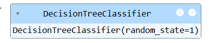
4: Defining the Model
Using DecisionTreeClassifier from sklearn.tree create an object for the Decision Tree Classifier.
clf = DecisionTreeClassifier(random_state=1)
5: Training the Model
Apply the fit method to match the classifier to the training set of data.
clf.fit(X_train, y_train)
Output:
6: Making Predictions
Apply the predict method to the test data and use the trained model to create predictions.
y_pred = clf.predict(X_test)

accuracy = accuracy_score(y_test, y_pred)
print(f'Accuracy: {accuracy}')
Output:
Accuracy: 0.9555555555555556
7: Hyperparameter Tuning with Decision Tree Classifier using GridSearchCV
Hyperparameters are configuration settings that control how a decision tree model learns from data.
- Proper tuning helps improve accuracy, reduce overfitting and enhance model generalization.
- Well-chosen hyperparameters allow the model to balance complexity and performance effectively.
- Common tuning techniques include Grid Search, Random Search and Bayesian Optimization which evaluate multiple parameter combinations to find the optimal configuration.
Refer: How to tune a Decision Tree in Hyperparameter tuning?
Let's make use of Scikit-Learn's GridSearchCV to find the best combination of of hyperparameter values. The code is as follows:
from sklearn.model_selection import GridSearchCV

param_grid = {
    'max_depth': range(1, 10, 1),
    'min_samples_leaf': range(1, 20, 2),
    'min_samples_split': range(2, 20, 2),
    'criterion': ["entropy", "gini"]
}

tree = DecisionTreeClassifier(random_state=1)

grid_search = GridSearchCV(estimator=tree, param_grid=param_grid,
                           cv=5, verbose=True)
grid_search.fit(X_train, y_train)

print("best accuracy", grid_search.best_score_)
print(grid_search.best_estimator_)
Output:
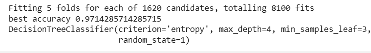
Here we defined the parameter grid with a set of hyperparameters and a list of possible values. The GridSearchCV evaluates the different hyperparameter combinations for the Decision Tree Classifier and selects the best combination of hyperparameters based on the performance across all k folds.
8: Visualizing the Decision Tree Classifier
Decision Tree visualization is used to interpret and comprehend model's choices. We'll plot feature importance obtained from the Decision Tree model to see which features have the greatest predictive power. Here we fetch the best estimator obtained from the GridSearchCV as the decision tree classifier.
from sklearn.tree import plot_tree
import matplotlib.pyplot as plt

tree_clf = grid_search.best_estimator_

plt.figure(figsize=(18, 15))
plot_tree(tree_clf, filled=True, feature_names=iris.feature_names,
          class_names=iris.target_names)
plt.show()
Output:
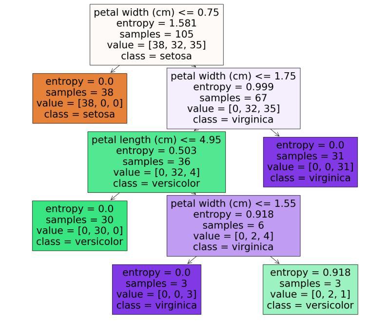
We can see that it start from the root node (depth 0 at the top).
- The root node checks whether the flower petal width is less than or equal to 0.75. If it is then we move to the root's left child node (depth1, left). Here the left node doesn't have any child nodes so the classifier will predict the class for that node as setosa.
- If the petal width is greater than 0.75 then we must move down to the root's right child node (depth 1, right). Here the right node is not a leaf node, so node check for the condition until it reaches the leaf node.
By using hyperparameter tuning methods like GridSearchCV we can optimize their performance.
