Mathematics | Beta Distribution Model
Last Updated :
03 Sep, 2024
The Beta Distribution is a continuous probability distribution defined on the interval [0, 1], widely used in statistics and various fields for modeling random variables that represent proportions or probabilities. It is particularly useful when dealing with scenarios where the outcomes are bounded within a specific range, such as success rates, probabilities, and proportions in Bayesian inference, decision theory, and reliability analysis. The flexibility of the Beta Distribution allows it to take on various shapes depending on its parameters, making it a versatile tool in mathematical modeling.
The beta distribution is used to model continuous random variables whose range is between 0 and 1. For example, in Bayesian analyses, the beta distribution is often used as a prior distribution of the parameter p (which is bounded between 0 and 1) of the binomial distribution (see, e.g., Novick and Jackson, 1974).
Definition of the Beta Distribution
The Beta Distribution is parameterized by two positive shape parameters, α, and β, which determine the shape of the distribution.
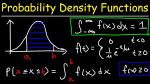
The probability density function (PDF) of the Beta Distribution for a random variable X on the interval [0, 1] is given by:
f(x;α,β)= xα−1 (1−x)β−1 / B(α,β)
where 𝐵(𝛼,𝛽) is the Beta function, defined as:
B(α,β)=∫01 tα−1 (1−t)β−1 dt
This function serves as a normalization constant ensuring that the total probability over the interval [0, 1] equals 1.
Properties of the Beta Distribution
The Beta Distribution exhibits several key properties, which are essential for understanding its behavior and applications.
Probability Density Function (PDF)
The Probability Density Function (PDF) of the Beta Distribution describes the likelihood of a random variable X taking on a specific value within the interval [0, 1].
The shape of the PDF is influenced by the parameters α and 𝛽. Depending on these parameters, the distribution can be uniform, U-shaped, J-shaped, or bell-shaped, making it adaptable to various situations.
 Probability Density Function
Cumulative Distribution Function (CDF)
The Cumulative Distribution Function (CDF) of the Beta Distribution, denoted as F(x;α,β), represents the probability that the random variable X is less than or equal to a specific value 𝑥.
It is computed as the integral of the PDF from 0 to 𝑥:
F(x;α,β)=∫0x f(t;α,β)dt
The CDF provides a way to calculate the probability of observing a value within a certain range, making it useful in hypothesis testing and confidence interval estimation.
Moments: Mean, Variance, Skewness, and Kurtosis
The moments of the Beta Distribution, including the mean, variance, skewness, and kurtosis, provide essential insights into the distribution's characteristics.
Mean:
The mean 𝐸[𝑋] of the Beta Distribution, which represents the central location or average value, is calculated as:
𝐸[𝑋]=𝛼/𝛼+𝛽
This formula shows that the mean is influenced by the relative values of the shape parameters 𝛼 and 𝛽. When 𝛼 equals 𝛽, the mean is 0.5, indicating a symmetric distribution centered around 0.5.
Variance:
The variance
Var(𝑋) measures the dispersion or spread of the distribution around the mean:
Var(𝑋)=𝛼𝛽 / (𝛼+𝛽)2(𝛼+𝛽+1)
A smaller variance indicates that the distribution is more concentrated around the mean, while a larger variance suggests a wider spread.
Skewness:
Skewness quantifies the asymmetry of the distribution. For the Beta Distribution, skewness is given by:
Skewness (𝑋)=2(𝛽−𝛼)√𝛼+𝛽+1/(𝛼+𝛽+2)√𝛼𝛽
- If 𝛼=𝛽, the distribution is symmetric (skewness = 0).
- If 𝛼>𝛽, the distribution is skewed to the left (negative skewness).
- If 𝛽>𝛼, the distribution is skewed to the right (positive skewness).
Kurtosis:
Kurtosis measures the "tailedness" or the concentration of data in the tails of the distribution:
Kurtosis(𝑋)=6[(𝛼−𝛽)2(𝛼+𝛽+1)𝛼𝛽(𝛼+𝛽+2)] / 𝛼𝛽(𝛼+𝛽+2)(𝛼+𝛽+3)
The kurtosis of the Beta Distribution can vary significantly based on the parameters 𝛼 and 𝛽, influencing the peak and tail behavior of the distribution.
Suppose an event can occur several times within a given unit of time. When the total number of occurrences of the event is unknown, we can think of it as a random variable. When a random variable X takes on values on the interval from 0 to 1, one choice of a probability density is the beta distribution whose probability density function is given by as follows.
Representation of probability density function -
f(x) = \frac{1}{\Beta(m.n)}x^{m-1}(1-x)^{n-1}
It will be applicable only when the given below given condition will pass.
x > 0, m >0, n >0.
f(x) = 0 , Otherwise
Here, you will see the meaning of function as you have shown in representation of probability density function where, B(m.n) is the value of the beta function.
Representation of B(m.n) -
\Beta(m,n) = \int^{1}_{0} x^{m- 1}(1-x)^{n-1}dx = \Beta(n,m)
Integrating it by parts, we will get the following expression as given below.
\Beta(m,n) = \frac{\Gamma(m)\Gamma(n)}{\Gamma(m+n)}
Where, Γ(x) is the gamma function of x, calculated as -
Γ(x) = (x-1)Γ(x-1) for x>1
=> \Gamma(x) = (x-1)! when x is an integer
The random variable X is represented as follows.
Representation of random variable X -
X ~ BETA(m,n)
Expected Value:
The Expected Value of the Beta distribution can be found by summing up products of Values with their respective probabilities.
\mu = E(X) = \int^{\infty}_{-\infty} x.f(x) dx
\mu = \frac{1}{\Beta(m,n)} \int^{1}_{0}x. x^{m - 1}(1-x)^{n-1} dx
\mu = \frac{1}{\Beta(m,n)} \int^{1}_{0} x^{m}(1-x)^{n-1} dx
Upon using the value of beta function, we will get the following expression a follows.
\mu = \frac{1}{\Beta(m,n)} \Beta(m+1,n)
but, \Beta(m,n) = \frac{\Gamma(m)\Gamma(n)}{\Gamma(m+n)}
also, \Beta(m+1,n) = \frac{\Gamma(m+1)\Gamma(n)}{\Gamma(m+n+1)}
=> \mu = \frac{\Gamma(m+1)\Gamma(n)}{\Gamma(m+n+1)} * \frac{\Gamma(m+n)}{\Gamma(m)\Gamma(n)}
Upon using the property of gamma function, that is Γ(x) = (x-1)!, we will get the following expression as follows.
So, E(x) = \frac{m! (n-1)! (m+n-1)!}{(m-1)! (n-1)! (m+n)!}
here, m, n -> integers
where provided m and n are integers.
Variance and Standard Deviation
The Variance of the Beta distribution can be found using the Variance Formula.
σ^2 = E( X − μ )^2 = E( X^2 ) − μ^2
E(X^2) = \int^{\infty}_{-\infty} x^2.f(x) dx
E(X^2) = \int^{1}_{0}\frac{1}{\Beta(m,n)}x^2. x^{m - 1}(1-x)^{n-1} dx
E(X^2) = \frac{1}{\Beta(m,n)}\int^{1}_{0}x^{m + 1}(1-x)^{n-1} dx
Upon using the value of beta function, we will get the following expression as follows.
E(X^2) = \frac{1}{\Beta(m,n)} \Beta(m+2,n+2)
but, \Beta(m,n) = \frac{\Gamma(m)\Gamma(n)}{\Gamma(m+n)}
also, \Beta(m+1,n) = \frac{\Gamma(m+2)\Gamma(n)}{\Gamma(m+n+2)}
=> \mu = \frac{\Gamma(m+2)\Gamma(n)}{\Gamma(m+n+2)} * \frac{\Gamma(m+n)}{\Gamma(m)\Gamma(n)}
Upon using the property of gamma function, that is Γ(x) = (x-1)!, we will get the following expression as follows.
E(X^2) = \frac{(m+1)!(n-1)!(m+n-1)!}{(m+n+1)!(m-1)!(n-1)!}
E(X^2) = \frac{m(m+1)}{(m+n+1)(m+n)}
So, Var(X) = E(X^2) - \mu^2
Var(X) = \frac{m(m+1)}{(m+n+1)(m+n)} - \frac{m^2}{(m+n)^2}
Var(X) = \sigma^2= \frac{m.n}{(m+n+1)(m+n)^2}
Standard Deviation is given by as follows.
\sigma = \sqrt{\frac{m.n}{(m+n+1)(m+n)^2}} = \frac{1}{(m+ n)}\sqrt{\frac{m.n}{(m+n+1)}}
Example -
In a certain county, the proportion of highway sections requiring repairs in any given year is a random variable having the beta distribution with m = 3 and n = 2.
(a) On the average, what percentage of the highway sections require repairs in any given year?
(b) Find the probability that at most half of the highway sections will require repairs in any given year.
Solution -
(a) \mu = \frac{3}{3+2} = 0.60
which means that on the average 60% of the highway sections require repairs in any given year.
(b) Substituting m=3 and n=2 in the probability density function, and
using Γ(3) = 2! = 2, Γ(2) = 1! = 1, Γ(5) = 4! = 24,
we will get the following expression as follows.
f(x) = 12 x^2 (1 − x) for 0<x<1. Otherwise f(x) = 0
Thus, the desired probability is given by as follows.
\int^{\frac{1}{2}}_0 12x^2 (1-x) dx = \frac{5}{16}
Shape of the Beta Distribution
The shape of the Beta Distribution is determined by the parameters
𝛼 and 𝛽, allowing it to take on various forms:
Uniform Distribution:
When 𝛼=𝛽=1, the Beta Distribution becomes a uniform distribution on the interval [0, 1], meaning every value within this interval is equally likely.
Bell-Shaped Distribution:
When 𝛼>1 and 𝛽>1, the Beta Distribution takes on a bell-shaped, unimodal form. The peak of the distribution occurs at 𝛼−1 / 𝛼+𝛽−2, making it suitable for modeling distributions with a central tendency.
U-Shaped Distribution:
When 𝛼<1 and 𝛽<1, the distribution is U-shaped, with most of the probability mass concentrated at the boundaries 0 and 1. This form is useful for modeling extreme probabilities.
J-Shaped Distribution:
When 𝛼<1 and 𝛽>1, the distribution is skewed towards 0, resembling a J-shape.
When 𝛼>1 and 𝛽<1, the distribution is skewed towards 1, also taking on a J-shaped form.
Applications of the Beta Distribution
The Beta Distribution's versatility makes it valuable across various fields:
Bayesian Inference:
The Beta Distribution is frequently used as a prior distribution in Bayesian analysis, especially for modeling binary outcomes and probabilities. Its conjugate nature with the binomial distribution simplifies posterior calculations.
Project Management (PERT):
In project management, the Beta Distribution is used in the Program Evaluation and Review Technique (PERT) to model the distribution of task completion times. It helps in estimating the expected duration and the likelihood of meeting deadlines.
Reliability Engineering:
The Beta Distribution is applied to model the life expectancy and failure rates of systems and components, particularly when data is sparse or when modeling expert opinions.
Genetics and Population Studies:
The Beta Distribution is employed to model the distribution of allele frequencies in populations, providing insights into genetic diversity and evolutionary dynamics.
Quality Control:
In quality control processes, the Beta Distribution is used to model the distribution of defect rates, helping organizations understand and manage variability in production processes.
The Beta Distribution's ability to model proportions, probabilities, and bounded outcomes makes it a powerful tool in both theoretical and applied statistics.
Solved Examples on Beta Distribution Model
Example 1: For a Beta Distribution with parameters α = 2 and β = 5:
- Mean: Calculate using the formula
α / (α + β). Thus, the mean is 2 / (2 + 5) = 2 / 7 ≈ 0.286. - Variance: Use the formula
αβ / [(α + β)² (α + β + 1)]. Therefore, the variance is 2 * 5 / [7² * 8] = 10 / 49 * 8 ≈ 0.0255.
Example 2: In a survey with α = 3 and β = 7, find the probability that the proportion is less than 0.4:
- Solution: To find this, use the cumulative distribution function (CDF) of the Beta Distribution evaluated at 0.4 with the given parameters.
Example 3: For α = 4 and β = 4, compute the skewness:
- Skewness: Using the formula
2 (β - α) sqrt(α + β + 1) / [(α + β + 2) sqrt(αβ)], the skewness is 2 * (4 - 4) * sqrt(8) / [(10) * sqrt(16)] = 0 because α equals β.
Example 4: With α = 1 and β = 2, find the probability that X is between 0.2 and 0.5:
- Solution: Calculate the difference between the CDF values at 0.5 and 0.2 using the given parameters.
Example 5: For α = 5 and β = 3, compute the kurtosis:
- Kurtosis: Substitute α and β into the kurtosis formula and simplify to obtain the value.
Practice Problems
- Compute the mean and variance for a Beta Distribution with α = 7 and β = 3.
- Find the probability that X is less than 0.6 for a Beta Distribution with α = 4 and β = 5.
- Determine the skewness of a Beta Distribution with α = 2 and β = 6.
- For α = 6 and β = 2, calculate the probability that X is greater than 0.3.
- Find the kurtosis for a Beta Distribution with α = 3 and β = 8.
- Compute the mean for a Beta Distribution where α = 10 and β = 15.
- Calculate the variance of a Beta Distribution with α = 5 and β = 5.
- Determine the CDF value at x = 0.7 for α = 2 and β = 3.
- Find the probability that X is between 0.4 and 0.8 for α = 4 and β = 6.
- Compute the skewness of a Beta Distribution with α = 8 and β = 4.
Summary / Conclusion
The Beta Distribution is a powerful and flexible tool used in statistics to model random variables constrained within the interval [0, 1]. Its versatility, governed by the parameters α and β, allows it to model various shapes of distributions, from uniform to bell-shaped, U-shaped, and J-shaped. The distribution's mean, variance, skewness, and kurtosis provide deep insights into its behavior, making it suitable for diverse applications such as Bayesian inference, project management, reliability engineering, genetics, and quality control. Understanding these properties helps in effective modeling and analysis of bounded outcomes.
Similar Reads
Maths for Machine Learning Mathematics is the foundation of machine learning. Math concepts plays a crucial role in understanding how models learn from data and optimizing their performance. Before diving into machine learning algorithms, it's important to familiarize yourself with foundational topics, like Statistics, Probab
5 min read
Linear Algebra and Matrix
MatricesMatrices are key concepts in mathematics, widely used in solving equations and problems in fields like physics and computer science. A matrix is simply a grid of numbers, and a determinant is a value calculated from a square matrix.Example: \begin{bmatrix} 6 & 9 \\ 5 & -4 \\ \end{bmatrix}_{2
3 min read
Scalar and VectorScalar and Vector Quantities are used to describe the motion of an object. Scalar Quantities are defined as physical quantities that have magnitude or size only. For example, distance, speed, mass, density, etc.However, vector quantities are those physical quantities that have both magnitude and dir
8 min read
Add Two Matrices - PythonThe task of adding two matrices in Python involves combining corresponding elements from two given matrices to produce a new matrix. Each element in the resulting matrix is obtained by adding the values at the same position in the input matrices. For example, if two 2x2 matrices are given as:Two 2x2
3 min read
Python Program to Multiply Two MatricesGiven two matrices, we will have to create a program to multiply two matrices in Python. Example: Python Matrix Multiplication of Two-DimensionPythonmatrix_a = [[1, 2], [3, 4]] matrix_b = [[5, 6], [7, 8]] result = [[0, 0], [0, 0]] for i in range(2): for j in range(2): result[i][j] = (matrix_a[i][0]
5 min read
Vector OperationsVectors are fundamental quantities in physics and mathematics, that have both magnitude and direction. So performing mathematical operations on them directly is not possible. So we have special operations that work only with vector quantities and hence the name, vector operations. Thus, It is essent
8 min read
Product of VectorsVector operations are used almost everywhere in the field of physics. Many times these operations include addition, subtraction, and multiplication. Addition and subtraction can be performed using the triangle law of vector addition. In the case of products, vector multiplication can be done in two
5 min read
Scalar Product of VectorsTwo vectors or a vector and a scalar can be multiplied. There are mainly two kinds of products of vectors in physics, scalar multiplication of vectors and Vector Product (Cross Product) of two vectors. The result of the scalar product of two vectors is a number (a scalar). The common use of the scal
9 min read
Dot and Cross Products on VectorsA quantity that has both magnitude and direction is known as a vector. Various operations can be performed on such quantities, such as addition, subtraction, and multiplication (products), etc. Some examples of vector quantities are: velocity, force, acceleration, and momentum, etc.Vectors can be mu
8 min read
Transpose a matrix in Single line in PythonTranspose of a matrix is a task we all can perform very easily in Python (Using a nested loop). But there are some interesting ways to do the same in a single line. In Python, we can implement a matrix as a nested list (a list inside a list). Each element is treated as a row of the matrix. For examp
4 min read
Transpose of a MatrixA Matrix is a rectangular arrangement of numbers (or elements) in rows and columns. It is often used in mathematics to represent data, solve systems of equations, or perform transformations. A matrix is written as:A = \begin{bmatrix} 1 & 2 & 3\\ 4 & 5 & 6 \\ 7 & 8 & 9\end{bma
11 min read
Adjoint and Inverse of a MatrixGiven a square matrix, find the adjoint and inverse of the matrix. We strongly recommend you to refer determinant of matrix as a prerequisite for this. Adjoint (or Adjugate) of a matrix is the matrix obtained by taking the transpose of the cofactor matrix of a given square matrix is called its Adjoi
15+ min read
How to inverse a matrix using NumPyIn this article, we will see NumPy Inverse Matrix in Python before that we will try to understand the concept of it. The inverse of a matrix is just a reciprocal of the matrix as we do in normal arithmetic for a single number which is used to solve the equations to find the value of unknown variable
3 min read
Program to find Determinant of a MatrixThe determinant of a Matrix is defined as a special number that is defined only for square matrices (matrices that have the same number of rows and columns). A determinant is used in many places in calculus and other matrices related to algebra, it actually represents the matrix in terms of a real n
15+ min read
Program to find Normal and Trace of a matrixGiven a 2D matrix, the task is to find Trace and Normal of matrix.Normal of a matrix is defined as square root of sum of squares of matrix elements.Trace of a n x n square matrix is sum of diagonal elements. Examples : Input : mat[][] = {{7, 8, 9}, {6, 1, 2}, {5, 4, 3}}; Output : Normal = 16 Trace =
6 min read
Data Science | Solving Linear EquationsLinear Algebra is a very fundamental part of Data Science. When one talks about Data Science, data representation becomes an important aspect of Data Science. Data is represented usually in a matrix form. The second important thing in the perspective of Data Science is if this data contains several
8 min read
Data Science - Solving Linear Equations with PythonA collection of equations with linear relationships between the variables is known as a system of linear equations. The objective is to identify the values of the variables that concurrently satisfy each equation, each of which is a linear constraint. By figuring out the system, we can learn how the
4 min read
System of Linear EquationsIn mathematics, a system of linear equations consists of two or more linear equations that share the same variables. These systems often arise in real-world applications, such as engineering, physics, economics, and more, where relationships between variables need to be analyzed. Understanding how t
8 min read
System of Linear Equations in three variables using Cramer's RuleCramer's rule: In linear algebra, Cramer's rule is an explicit formula for the solution of a system of linear equations with as many equations as unknown variables. It expresses the solution in terms of the determinants of the coefficient matrix and of matrices obtained from it by replacing one colu
12 min read
Eigenvalues and EigenvectorsEigenvectors are the directions that remain unchanged during a transformation, even if they get longer or shorter. Eigenvalues are the numbers that indicate how much something stretches or shrinks during that transformation. These ideas are important in many areas of math and engineering, including
15+ min read
Applications of Eigenvalues and EigenvectorsEigenvalues and eigenvectors play a crucial role in a wide range of applications across engineering and science. Fields like control theory, vibration analysis, electric circuits, advanced dynamics, and quantum mechanics frequently rely on these concepts. One key application involves transforming ma
7 min read
How to compute the eigenvalues and right eigenvectors of a given square array using NumPY?In this article, we will discuss how to compute the eigenvalues and right eigenvectors of a given square array using NumPy library. Example: Suppose we have a matrix as: [[1,2], [2,3]] Eigenvalue we get from this matrix or square array is: [-0.23606798 4.23606798] Eigenvectors of this matrix are
2 min read
Statistics for Machine Learning
Descriptive StatisticStatistics is the foundation of data science. Descriptive statistics are simple tools that help us understand and summarize data. They show the basic features of a dataset, like the average, highest and lowest values and how spread out the numbers are. It's the first step in making sense of informat
5 min read
Measures of Central TendencyUsually, frequency distribution and graphical representation are used to depict a set of raw data to attain meaningful conclusions from them. However, sometimes, these methods fail to convey a proper and clear picture of the data as expected. Therefore, some measures, also known as Measures of Centr
5 min read
Measures of Dispersion | Types, Formula and ExamplesMeasures of Dispersion are used to represent the scattering of data. These are the numbers that show the various aspects of the data spread across multiple parameters.Let's learn about the measure of dispersion in statistics, its types, formulas, and examples in detail.Dispersion in StatisticsDisper
9 min read
Mean, Variance and Standard DeviationMean, Variance and Standard Deviation are fundamental concepts in statistics and engineering mathematics, essential for analyzing and interpreting data. These measures provide insights into data's central tendency, dispersion, and spread, which are crucial for making informed decisions in various en
10 min read
Calculate the average, variance and standard deviation in Python using NumPyNumpy in Python is a general-purpose array-processing package. It provides a high-performance multidimensional array object and tools for working with these arrays. It is the fundamental package for scientific computing with Python. Numpy provides very easy methods to calculate the average, variance
5 min read
Random VariableRandom variable is a fundamental concept in statistics that bridges the gap between theoretical probability and real-world data. A Random variable in statistics is a function that assigns a real value to an outcome in the sample space of a random experiment. For example: if you roll a die, you can a
10 min read
Difference between Parametric and Non-Parametric MethodsStatistical analysis plays a crucial role in understanding and interpreting data across various disciplines. Two prominent approaches in statistical analysis are Parametric and Non-Parametric Methods. While both aim to draw inferences from data, they differ in their assumptions and underlying princi
8 min read
Probability Distribution - Function, Formula, TableA probability distribution is a mathematical function or rule that describes how the probabilities of different outcomes are assigned to the possible values of a random variable. It provides a way of modeling the likelihood of each outcome in a random experiment.While a frequency distribution shows
15+ min read
Confidence IntervalA Confidence Interval (CI) is a range of values that contains the true value of something we are trying to measure like the average height of students or average income of a population.Instead of saying: “The average height is 165 cm.â€We can say: “We are 95% confident the average height is between 1
7 min read
Covariance and CorrelationCovariance and correlation are the two key concepts in Statistics that help us analyze the relationship between two variables. Covariance measures how two variables change together, indicating whether they move in the same or opposite directions. Relationship between Independent and dependent variab
5 min read
Program to Find Correlation CoefficientThe correlation coefficient is a statistical measure that helps determine the strength and direction of the relationship between two variables. It quantifies how changes in one variable correspond to changes in another. This coefficient, sometimes referred to as the cross-correlation coefficient, al
8 min read
Robust CorrelationCorrelation is a statistical tool that is used to analyze and measure the degree of relationship or degree of association between two or more variables. There are generally three types of correlation: Positive correlation: When we increase the value of one variable, the value of another variable inc
8 min read
Normal Probability PlotThe probability plot is a way of visually comparing the data coming from different distributions. These data can be of empirical dataset or theoretical dataset. The probability plot can be of two types:P-P plot: The (Probability-to-Probability) p-p plot is the way to visualize the comparing of cumul
3 min read
Quantile Quantile plotsThe quantile-quantile( q-q plot) plot is a graphical method for determining if a dataset follows a certain probability distribution or whether two samples of data came from the same population or not. Q-Q plots are particularly useful for assessing whether a dataset is normally distributed or if it
8 min read
True Error vs Sample ErrorTrue Error The true error can be said as the probability that the hypothesis will misclassify a single randomly drawn sample from the population. Here the population represents all the data in the world. Let's consider a hypothesis h(x) and the true/target function is f(x) of population P. The proba
3 min read
Bias-Variance Trade Off - Machine LearningIt is important to understand prediction errors (bias and variance) when it comes to accuracy in any machine-learning algorithm. There is a tradeoff between a model’s ability to minimize bias and variance which is referred to as the best solution for selecting a value of Regularization constant. A p
3 min read
Hypothesis TestingHypothesis testing compares two opposite ideas about a group of people or things and uses data from a small part of that group (a sample) to decide which idea is more likely true. We collect and study the sample data to check if the claim is correct.Hypothesis TestingFor example, if a company says i
9 min read
T-testAfter learning about the Z-test we now move on to another important statistical test called the t-test. While the Z-test is useful when we know the population variance. The t-test is used to compare the averages of two groups to see if they are significantly different from each other. Suppose you wa
6 min read
Paired T-Test - A Detailed OverviewStudent’s t-test or t-test is the statistical method used to determine if there is a difference between the means of two samples. The test is often performed to find out if there is any sampling error or unlikeliness in the experiment. This t-test is further divided into 3 types based on your data a
5 min read
P-value in Machine LearningP-value helps us determine how likely it is to get a particular result when the null hypothesis is assumed to be true. It is the probability of getting a sample like ours or more extreme than ours if the null hypothesis is correct. Therefore, if the null hypothesis is assumed to be true, the p-value
6 min read
F-Test in StatisticsF test is a statistical test that is used in hypothesis testing that determines whether the variances of two samples are equal or not. The article will provide detailed information on f test, f statistic, its calculation, critical value and how to use it to test hypotheses. To understand F test firs
6 min read
Z-test : Formula, Types, ExamplesA Z-test is a type of hypothesis test that compares the sample’s average to the population’s average and calculates the Z-score and tells us how much the sample average is different from the population average by looking at how much the data normally varies. It is particularly useful when the sample
8 min read
Residual Leverage Plot (Regression Diagnostic)In linear or multiple regression, it is not enough to just fit the model into the dataset. But, it may not give the desired result. To apply the linear or multiple regression efficiently to the dataset. There are some assumptions that we need to check on the dataset that made linear/multiple regress
5 min read
Difference between Null and Alternate HypothesisHypothesis is a statement or an assumption that may be true or false. There are six types of hypotheses mainly the Simple hypothesis, Complex hypothesis, Directional hypothesis, Associative hypothesis, and Null hypothesis. Usually, the hypothesis is the start point of any scientific investigation, I
3 min read
Mann and Whitney U testMann and Whitney's U-test or Wilcoxon rank-sum testis the non-parametric statistic hypothesis test that is used to analyze the difference between two independent samples of ordinal data. In this test, we have provided two randomly drawn samples and we have to verify whether these two samples is from
5 min read
Wilcoxon Signed Rank TestThe Wilcoxon Signed Rank Test is a non-parametric statistical test used to compare two related groups. It is often applied when the assumptions for the paired t-test (such as normality) are not met. This test evaluates whether there is a significant difference between two paired observations, making
5 min read
Kruskal Wallis TestThe Kruskal-Wallis test (H test) is a nonparametric statistical test used to compare three or more independent groups to determine if there are statistically significant differences between them. It is an extension of the Mann-Whitney U test, which is used for comparing two groups.Unlike the one-way
4 min read
Friedman TestThe Friedman Test is a non-parametric statistical test used to detect differences in treatments across multiple test attempts. It is often used when the data is in the form of rankings or ordinal data, and when you have more than two related groups or repeated measures. The Friedman test is the non-
6 min read
Probability Class 10 Important QuestionsProbability is a fundamental concept in mathematics for measuring of chances of an event happening By assigning numerical values to the chances of different outcomes, probability allows us to model, analyze, and predict complex systems and processes.Probability Formulas for Class 10 It says the poss
4 min read
Probability and Probability Distributions
Mathematics - Law of Total ProbabilityProbability theory is the branch of mathematics concerned with the analysis of random events. It provides a framework for quantifying uncertainty, predicting outcomes, and understanding random phenomena. In probability theory, an event is any outcome or set of outcomes from a random experiment, and
12 min read
Bayes's Theorem for Conditional ProbabilityBayes's Theorem for Conditional Probability: Bayes's Theorem is a fundamental result in probability theory that describes how to update the probabilities of hypotheses when given evidence. Named after the Reverend Thomas Bayes, this theorem is crucial in various fields, including engineering, statis
9 min read
Uniform Distribution in Data ScienceUniform Distribution also known as the Rectangular Distribution is a type of Continuous Probability Distribution where all outcomes in a given interval are equally likely. Unlike Normal Distribution which have varying probabilities across their range, Uniform Distribution has a constant probability
5 min read
Binomial Distribution in Data ScienceBinomial Distribution is used to calculate the probability of a specific number of successes in a fixed number of independent trials where each trial results in one of two outcomes: success or failure. It is used in various fields such as quality control, election predictions and medical tests to ma
7 min read
Poisson Distribution in Data SciencePoisson Distribution is a discrete probability distribution that models the number of events occurring in a fixed interval of time or space given a constant average rate of occurrence. Unlike the Binomial Distribution which is used when the number of trials is fixed, the Poisson Distribution is used
7 min read
Uniform Distribution | Formula, Definition and ExamplesA Uniform Distribution is a type of probability distribution in which every outcome in a given range is equally likely to occur. That means there is no bias—no outcome is more likely than another within the specified set.It is also known as rectangular distribution (continuous uniform distribution).
11 min read
Exponential DistributionThe Exponential Distribution is one of the most commonly used probability distributions in statistics and data science. It is widely used to model the time or space between events in a Poisson process. In simple terms, it describes how long you have to wait before something happens, like a bus arriv
3 min read
Normal Distribution in Data ScienceNormal Distribution also known as the Gaussian Distribution or Bell-shaped Distribution is one of the widely used probability distributions in statistics. It plays an important role in probability theory and statistics basically in the Central Limit Theorem (CLT). It is characterized by its bell-sha
6 min read
Mathematics | Beta Distribution ModelThe Beta Distribution is a continuous probability distribution defined on the interval [0, 1], widely used in statistics and various fields for modeling random variables that represent proportions or probabilities. It is particularly useful when dealing with scenarios where the outcomes are bounded
11 min read
Gamma Distribution Model in MathematicsIntroduction : Suppose an event can occur several times within a given unit of time. When the total number of occurrences of the event is unknown, we can think of it as a random variable. Now, if this random variable X has gamma distribution, then its probability density function is given as follows
2 min read
Chi-Square Test for Feature Selection - Mathematical ExplanationOne of the primary tasks involved in any supervised Machine Learning venture is to select the best features from the given dataset to obtain the best results. One way to select these features is the Chi-Square Test. Mathematically, a Chi-Square test is done on two distributions two determine the lev
4 min read
Student's t-distribution in StatisticsAs we know normal distribution assumes two important characteristics about the dataset: a large sample size and knowledge of the population standard deviation. However, if we do not meet these two criteria, and we have a small sample size or an unknown population standard deviation, then we use the
10 min read
Python - Central Limit TheoremCentral Limit Theorem (CLT) is a foundational principle in statistics, and implementing it using Python can significantly enhance data analysis capabilities. Statistics is an important part of data science projects. We use statistical tools whenever we want to make any inference about the population
7 min read
Limits, Continuity and DifferentiabilityLimits, Continuity, and Differentiation are fundamental concepts in calculus. They are essential for analyzing and understanding function behavior and are crucial for solving real-world problems in physics, engineering, and economics.Table of ContentLimitsKey Characteristics of LimitsExample of Limi
10 min read
Implicit DifferentiationImplicit Differentiation is the process of differentiation in which we differentiate the implicit function without converting it into an explicit function. For example, we need to find the slope of a circle with an origin at 0 and a radius r. Its equation is given as x2 + y2 = r2. Now, to find the s
5 min read
Calculus for Machine Learning
Partial Derivatives in Engineering MathematicsPartial derivatives are a basic concept in multivariable calculus. They convey how a function would change when one of its input variables changes, while keeping all the others constant. This turns out to be particularly useful in fields such as physics, engineering, economics, and computer science,
10 min read
Advanced DifferentiationDerivatives are used to measure the rate of change of any quantity. This process is called differentiation. It can be considered as a building block of the theory of calculus. Geometrically speaking, the derivative of any function at a particular point gives the slope of the tangent at that point of
8 min read
How to find Gradient of a Function using Python?The gradient of a function simply means the rate of change of a function. We will use numdifftools to find Gradient of a function. Examples: Input : x^4+x+1 Output :Gradient of x^4+x+1 at x=1 is 4.99 Input :(1-x)^2+(y-x^2)^2 Output :Gradient of (1-x^2)+(y-x^2)^2 at (1, 2) is [-4. 2.] Approach: For S
2 min read
Optimization techniques for Gradient DescentGradient Descent is a widely used optimization algorithm for machine learning models. However, there are several optimization techniques that can be used to improve the performance of Gradient Descent. Here are some of the most popular optimization techniques for Gradient Descent: Learning Rate Sche
4 min read
Higher Order DerivativesHigher order derivatives refer to the derivatives of a function that are obtained by repeatedly differentiating the original function.The first derivative of a function, f′(x), represents the rate of change or slope of the function at a point.The second derivative, f′′(x), is the derivative of the f
6 min read
Taylor SeriesA Taylor series represents a function as an infinite sum of terms, calculated from the values of its derivatives at a single point.Taylor series is a powerful mathematical tool used to approximate complex functions with an infinite sum of terms derived from the function's derivatives at a single poi
8 min read
Application of Derivative - Maxima and MinimaDerivatives have many applications, like finding rate of change, approximation, maxima/minima and tangent. In this section, we focus on their use in finding maxima and minima.Note: If f(x) is a continuous function, then for every continuous function on a closed interval has a maximum and a minimum v
6 min read
Absolute Minima and MaximaAbsolute Maxima and Minima are the maximum and minimum values of the function defined on a fixed interval. A function in general can have high values or low values as we move along the function. The maximum value of the function in any interval is called the maxima and the minimum value of the funct
11 min read
Optimization for Data ScienceFrom a mathematical foundation viewpoint, it can be said that the three pillars for data science that we need to understand quite well are Linear Algebra, Statistics and the third pillar is Optimization which is used pretty much in all data science algorithms. And to understand the optimization conc
5 min read
Unconstrained Multivariate OptimizationWikipedia defines optimization as a problem where you maximize or minimize a real function by systematically choosing input values from an allowed set and computing the value of the function. That means when we talk about optimization we are always interested in finding the best solution. So, let sa
4 min read
Lagrange Multipliers | Definition and ExamplesIn mathematics, a Lagrange multiplier is a potent tool for optimization problems and is applied especially in the cases of constraints. Named after the Italian-French mathematician Joseph-Louis Lagrange, the method provides a strategy to find maximum or minimum values of a function along one or more
8 min read
Lagrange's InterpolationWhat is Interpolation? Interpolation is a method of finding new data points within the range of a discrete set of known data points (Source Wiki). In other words interpolation is the technique to estimate the value of a mathematical function, for any intermediate value of the independent variable. F
7 min read
Linear Regression in Machine learningLinear regression is a type of supervised machine-learning algorithm that learns from the labelled datasets and maps the data points with most optimized linear functions which can be used for prediction on new datasets. It assumes that there is a linear relationship between the input and output, mea
15+ min read
Ordinary Least Squares (OLS) using statsmodelsOrdinary Least Squares (OLS) is a widely used statistical method for estimating the parameters of a linear regression model. It minimizes the sum of squared residuals between observed and predicted values. In this article we will learn how to implement Ordinary Least Squares (OLS) regression using P
3 min read
Regression in Machine Learning