Pivot Table Slicers in Excel

Slicers are visual filters in Excel that allow us to quickly and easily filter data in a Pivot Table or Pivot Chart by clicking on the items we want to see. Found in the Analyze tab of PivotTable Tools, they provide a more intuitive and user-friendly alternative to traditional drop-down filters.

They act as clickable buttons representing data fields and are useful when working with multiple columns, enabling dynamic and interactive control over the data displayed. In this article, we will see what pivot table slicers are and its core concepts.

How to Insert a Pivot Table Slicer?

Follow the below steps to insert a Pivot table slicer:

Step 1: Create a Pivot table: Select the data we want to analyze and then create a Pivot table.

Step 2: Design the Pivot Table: Design the Pivot table by dragging the relevant fields to the "Rows", "Columns", "Values" or "Filters" area of the PivotTable Fields pane.

Step 3: Insert a Slicer: When our Pivot Table is ready, go to the "Pivot Table Analyze" or "Options" tab in the Excel ribbon. Click on "Insert Slicer" and a dialog box will appear, with all the fields available in the Pivot Table.

Step 4: Choose a Field for the Slicer: Select the field we want to use as a slicer and click "OK".

Working with Slicers

Let’s understand how slicers work with an example. Imagine we have an IMDb dataset containing all movies released worldwide in 2016 including details like ratings, budget, gross revenue, country and genre. Now we want to find the total budget of movies by country, filtered by genre. For example the budget of comedy movies in the U.S.A and the U.K.

We can filter this data in two ways:

1. Using the Pivot Table filter: Drag the Genre field into the filter box in the Pivot Table field list and select the desired genres.

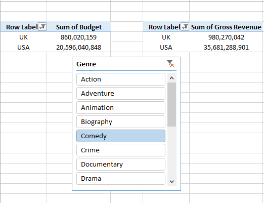
2. Using a slicer: Insert a slicer for the Genre field and click on the genres we want to filter by.

Both methods give the same results but slicers offer a more user-friendly and interactive way to filter data.

To select multiple genres in a slicer helps the Multi-select option or hold the Shift key while clicking the genres. For example, selecting both comedy and crime genres will show the total budget of those films in the U.S.A and U.K.

Formatting Slicers

When you insert a slicer, a new Slicer Tools menu appears in the ribbon which offers various options to customize our slicer’s appearance.

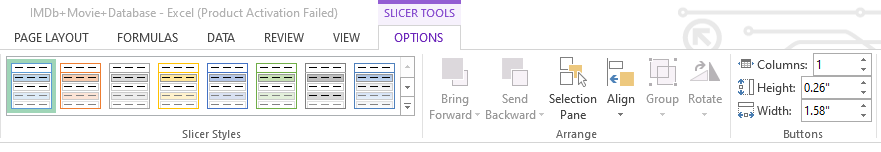
1. If our slicer contains many items, we can increase the number of columns to make it wider and display the items more neatly.

2. Additional formatting options are available under Slicer Settings where we can:

• Choose to show or hide the slicer header.
• Sort the slicer items in ascending or descending order.
• Adjust other display preferences to suit our needs.

How to Adjust Slicers in Excel?

After inserting slicers we may want to move, resize or customize them to fit our worksheet and improve usability. Excel provides several options to help us do this easily.

1. Moving a Slicers

To move a Slicer to a new location on the same worksheet, follow these steps:

1. Point to the Slicer's border or any empty part of the Slicer.
2. When the pointer changes to a 4-headed arrow, drag the slicers to their new position.

2. Resizing a Slicer

Follow the steps to resize a Slicer to make it larger or smaller:

1. Click on the slicer to select it.
2. Point to one of the sizing handles on its border.
3. When the cursor changes to a two-headed arrow, drag inward or outward to adjust the size.

3. Change Slicer Style

Excel has some built-in styles similar to Pivot Tables. To change the style:

1. Click on an empty part of the Slicer to select it.
2. On the Excel Ribbon, go to the "Slicer" tab.
3. In the "Slicer Styles" group, click on one of the visible styles to apply it to the Slicer.

4. Change Slicer Settings

We can modify various slicer settings to control its appearance and behavior:

1. Sort Order

• Step 1: Right-click on the Slicer and click "Slicer Settings".
• Step 2: In the "Item Sorting and Filtering" section, select "Ascending " or "Descending" as per our preference.
• Step 3: Click "Ok" to apply changes.

2. Change Slicer Captions:

• Step 1: Right-click on the Slicer and Click "Slicer Settings".
• Step 2: In the "Header" Section, type the desired caption text to replace the existing caption.
• Step 3: Click "ok" to save the changes.

5. Multiple Slicers

• We can insert multiple slicers if we want to filter our data based on two columns. Each of the slicers tells the pivot table what sub-set of data to use for calculating the numbers.
• For eg: In our example of the IMDb movies database that we took above if we want to filter our data on the basis of genre and language. i.e. If we want to calculate the budget of all the Hindi movies of comedy genre in the U.S.A and U.K then we insert two slicers, one on the basis of genre, the other on the basis of language.

So from the picture above, we can see that there are no Hindi comedy films in the U.K.

Linking a Slicer to Multiple Pivot Tables

We can link our slicer to multiple pivot tables which can build a very interactive dashboard. To do so follow the below steps:

Step 1: Right-click on the slicer and select the option of Report Connections.

Step 2: After that, we will see a menu like this.

Step 3: Now select all the table names on which we want our slicer to work.

For example, using the IMDb movies dataset we might want the slicer to filter both the budget and gross revenue pivot tables simultaneously for all comedy films in the U.S.A and U.K. Linking the slicer helps it to update both tables at once.

So here our slicer works on both the pivot tables.

Advantages of Using Pivot Table Slicers

Slicers offer several key benefits that make working with Pivot Tables easier and more efficient:

1. User-Friendly Data Exploration: Slicers provide an intuitive, visual way to explore and analyze data which helps in allowing users to filter data quickly without needing complex filtering tools.
2. Interactive Data Analysis: Users can instantly update their Pivot Table by changing slicer selections helps in offering real-time insights into the data.
3. Enhanced Visual Clarity: Slicers add a visual layer to Pivot Tables helps in making it easier to see which filters are applied and improving the overall data presentation.
4. Consistency Across Pivot Table: Slicers help maintain a consistent design across multiple Pivot Tables in the same workbook helps in creating a unified and standardized user experience.
5. Easy to Use and Customize: Inserting and customizing slicers is simple with no special training required. We can adjust their styles, sizes and layouts to fit our design preferences.

Using slicers makes data feel smooth and straightforward which helps in turning a usually boring task into something we actually enjoy doing.