Clustering Algorithms - Kmeans,Min ALgorithm

Clustering Algorithms
By
Sharmila Chidaravalli
Assistant Professor
Department of ISE
Global Academy of Technology

Introduction to Clustering Approaches
Cluster analysis is the fundamental task of unsupervised learning.
Unsupervised learning involves exploring the given dataset.
Cluster analysis is a technique of partitioning a collection of unlabelled
objects that have many attributes into meaningful disjoint groups or clusters.
This is done using a trial and error approach as there are no supervisors
available as in classification.
The characteristic of clustering is that the objects in the clusters or groups are
similar to each other within the clusters while differ from the objects in other
clusters significantly.
The input for cluster analysis is examples or samples. These are known as
objects, data points or data instances.
All the samples or objects with no labels associated with them are called
unlabelled.
The output is the set of clusters (or groups) of similar data if it exists in the
input.

Differences between Classification and Clustering

Applications of Clustering
1. Grouping based on customer buying patterns
2. Profiling of customers based on lifestyle
3. In information retrieval applications (like retrieval of a document from a collection of documents)
4. Identifying the groups of genes that influence a disease
5. Identification of organs that are similar in physiology functions
6. Taxonomy of animals, plants in Biology
7. Clustering based on purchasing behaviour and demography
8. Document indexing
9. Data compression by grouping similar objects and finding duplicate objects

Advantages and Disadvantages of Clustering Algorithms

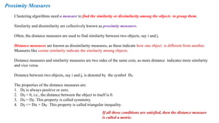
Proximity Measures
Clustering algorithms need a measure to find the similarity or dissimilarity among the objects to group them.
Similarity and dissimilarity are collectively known as proximity measures.
Often, the distance measures are used to find similarity between two objects, say i and j.
Distance measures are known as dissimilarity measures, as these indicate how one object is different from another.
Measures like cosine similarity indicate the similarity among objects.
Distance measures and similarity measures are two sides of the same coin, as more distance indicates more similarity
and vice versa.
Distance between two objects, say i and j, is denoted by the symbol Dij.
The properties of the distance measures are:
1. Dij is always positive or zero.
2. Dij = 0, i.e., the distance between the object to itself is 0.
3. Dij = Dji. This property is called symmetry.
4. Dij <= Dik + Dkj . This property is called triangular inequality.
If all these conditions are satisfied, then the distance measure
is called a metric.

Proximity Measures
Quantitative Variables
Euclidean Distance (L₂ norm)
•Definition: Measures the straight-line distance between two points in a Euclidean space.
•Formula:
•Advantages:
•Remains consistent with the addition of new objects.
•Disadvantages:
•Sensitive to unit changes.
•Computationally expensive due to square root operation.

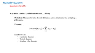
Proximity Measures
City Block Distance (Manhattan Distance, L₁ norm)
•Definition: Measures the total absolute difference across dimensions; like navigating a
grid in a city.
•Formula:
•Also known as:
• Manhattan distance
• Taxicab distance
• Absolute value distance

Proximity Measures
Chebyshev Distance (L∞ norm)
•Definition: The greatest absolute difference in any one dimension (max distance along any
coordinate axis).
•Formula:
•Also called:
• Maximum value distance
• Supremum distance

Proximity Measures
Minkowski Distance
This is called Minkowski distance.
r is a parameter.
r =1, the distance measure is called city block distance.
r = 2, the distance measure is called Euclidean distance.
r = ∞, then this is Chebyshev distance.

Proximity Measures
Binary Attributes
•These attributes take only two values: typically 0 and 1.
•Distance measures like Euclidean or Manhattan are not appropriate for binary data.
•Instead, we use contingency tables and set-based similarity measures.
Contingency Table for Binary Attributes
Let x and y be two binary vectors of length N. We define:
y = 0 y = 1
x = 0 a b
x = 1 c d
Where:
•a: Number of attributes where x = 0 and y = 0
•b: Number of attributes where x = 0 and y = 1
•c: Number of attributes where x = 1 and y = 0
•d: Number of attributes where x = 1 and y = 1
Total attributes = a+b+c+d

Proximity Measures
Binary Attributes
Simple Matching Coefficient (SMC)
•Definition: Measures how many attributes match in total (both 0–0 and 1–1).
•Formula:
Use: Suitable when both 0–0 and 1–1 matches are considered equally important.
Jaccard Coefficient
•Definition: Measures similarity only considering 1–1 matches.
•Formula:
•Use: Preferred when presence (1s) is more important than absence (0s).

Proximity Measures
Binary Attributes
Hamming Distance
•Definition:
The Hamming distance between two binary vectors or strings of equal length is the number of
positions at which the corresponding symbols differ.
•Use Cases:
•Binary strings
•Character sequences (e.g., DNA, words)
•Error detection and correction in digital communications
Examples:
•Binary Example
•x=(1,0,1)
•y=(1,1,0)
•Hamming Distance = 2 (differs in 2nd and 3rd positions)
•String Example
•"wood “ vs. "hood
•Hamming Distance = 1 (only 'w' vs 'h' differs)

Categorical Variables
Proximity Measures
In many cases, categorical values are used.
It is just a code or symbol to represent the values.
For example,
for the attribute Gender,
code 1 can be given to female and
code 0 can be given to male.
To calculate the distance between two objects represented by variables, we need to find only
whether they are equal or not.
This is given as:

Proximity Measures
Ordinal Variables
•Definition: Ordinal variables are categorical variables that have a meaningful order or ranking, but
the differences between values may not be equal.
•Examples:
•Job positions (Clerk < Supervisor < Manager < General Manager)
•Education levels (High School < Bachelor < Master < PhD)
•Ratings (Poor < Fair < Good < Excellent)
Distance Between Ordinal Values
To compute distances between ordinal variables, their ranked positions are first converted into
numerical values, then normalized.

Proximity Measures
Ordinal Variables
Example
Let:
•Clerk = 1
•Supervisor = 2
•Manager = 3
•General Manager = 4
Total levels n=4
Find the distance between:
•X = Clerk (1)
•Y = Manager (3)
Why Normalize?
•Normalizing by n−1 ensures that the distance lies between 0 and 1.
•Makes the distance measure comparable with other normalized distance measures in mixed data types.

For text classification, vectors are normally used.
Cosine similarity is a metric used to measure how similar the documents are irrespective of their size.
Cosine similarity measures the cosine of the angle between two vectors projected in a multi-
dimensional space.
The similarity function for vector objects can be defined as:
Proximity Measures
Vector Type Distance Measures

1. Consider the following data and calculate the Euclidean, Manhattan and Chebyshev distances:
(a) (2 3 4) and (1 5 6)
(b) (2 2 9) and (7 8 9)
(c ) (0,3) and (5,8)
2. Find cosine similarity, SMC and Jaccard coefficients for the following binary data:
(a) (1 0 1 1) and (1 1 0 0)
(b) (1 0 0 0 1) and (1 0 0 0 0 1) and (1 1 0 0 0)
3. Find Hamming distance for the following binary data:
(a) (1 1 1) and (1 0 0)
(b) (1 1 1 0 0) and (0 0 1 1 1)
4. Find the distance between:
(a) Employee ID: 1000 and 1001
(b) Employee name – John & John and John & Joan
5. Find the distance between:
(a) (Yellow, red, green) and (red, green, yellow)
(b) (bread, butter, milk) and (milk, sandwich, Tea)
6. If the given vectors are x = (1, 0, 0) and y = (1, 1, 1) then find the SMC and Jaccard coefficient?
7. If the given vectors are A = {1, 1, 0} and B = {0, 1, 1}, then what is the cosine similarity?

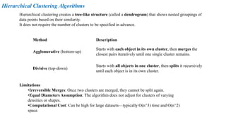
Hierarchical Clustering Algorithms
Hierarchical clustering creates a tree-like structure (called a dendrogram) that shows nested groupings of
data points based on their similarity.
It does not require the number of clusters to be specified in advance.
Method Description
Agglomerative (bottom-up)
Starts with each object in its own cluster, then merges the
closest pairs iteratively until one single cluster remains.
Divisive (top-down)
Starts with all objects in one cluster, then splits it recursively
until each object is in its own cluster.
Limitations
•Irreversible Merges: Once two clusters are merged, they cannot be split again.
•Equal Diameters Assumption: The algorithm does not adjust for clusters of varying
densities or shapes.
•Computational Cost: Can be high for large datasets—typically O(n^3) time and O(n^2)
space.

Hierarchical Clustering Algorithms
Agglomerative Clustering
1. Place each N sample or data instance into a separate cluster. So, initially N clusters are available.
2. Repeat the following steps until a single cluster is formed:
(a) Determine two most similar clusters.
(b) Merge the two clusters into a single cluster reducing the number of clusters as N–1
3. Choose resultant clusters of step 2 as result.
Dendrogram
•A visual representation of the clustering process.
•The height at which two clusters merge represents the distance (or dissimilarity) between them.
•By “cutting” the dendrogram at a certain level, we can decide on the number of final clusters.

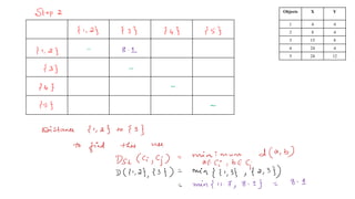
Single Linkage or MIN Algorithm
In single linkage algorithm, the smallest distance (x, y), where x is from one cluster and y is from
another cluster, is the distance between all possible pairs of the two groups or clusters (or simply the
smallest distance of two points where points are in different clusters) and is used for merging the
clusters.
This corresponds to finding of minimum spanning tree (MST) of a graph.
The distance between two points can be calculated
Here, DSL is the single linkage distance,
Ci, Cj are clusters
d (a, b) is the distance between the elements a and b.

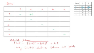
Problem : Consider the array of points. Apply single linkage algorithm.
Objects X Y
1 4 4
2 8 4
3 15 8
4 24 4
5 24 12

Objects X Y
1 4 4
2 8 4
3 15 8
4 24 4
5 24 12

Clustering Algorithms - Kmeans,Min ALgorithm

Complete Linkage or MAX or Clique
In complete linkage algorithm, the distance (x, y), (where x is from one cluster and y is from another cluster), is
the largest distance between all possible pairs of the two groups or clusters (or simply the largest distance of two
points where points are in different clusters) as given below.
It is used for merging the clusters.
Average Linkage
In case of an average linkage algorithm, the average distance of all pairs of points across the clusters is used to
form clusters. The average value computed between clusters ci, cj is given as follows:
Here, mi and mj are sizes of the clusters.

Mean-Shift Clustering Algorithm
Mean-shift is a non-parametric and hierarchical clustering algorithm.
This algorithm is also known as mode seeking algorithm or a sliding window algorithm.
There is no need for any prior knowledge of clusters or shape of the clusters present in
the dataset.
The algorithm slowly moves from its initial position towards the dense regions.
The algorithm uses a window, which is basically a weighting function.
The radius of the kernel is called bandwidth. The entire window is called a kernel.
The window is based on the concept of kernel density function and its aim is to find the
underlying data distribution.
The method of calculation of mean is dependent on the choice of windows.
If a Gaussian window is chosen, then every point is assigned a weight that decreases as
the distance from the kernel center increases.
Applications:
•Image segmentation
•Object tracking
•Feature space analysis

Algorithm
Step 1: Design a window.
Step 2: Place the window on a set of data points.
Step 3: Compute the mean for all the points that come under the window.
Step 4: Move the center of the window to the mean computed in step 3. Thus, the
window moves towards the dense regions. The movement to the dense region is
controlled by a mean shift vector.
The mean shift vector is given as:
Here, K is the number of points and Sk is the data points where the distance from
data points xi and centroid of the kernel x is within the radius of the sphere.
Then, the centroid is updated as
Step 5: Repeat the steps 3–4 for convergence. Once convergence is achieved, no
further points can be accommodated.

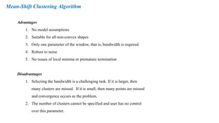
Advantages
1. No model assumptions
2. Suitable for all non-convex shapes
3. Only one parameter of the window, that is, bandwidth is required
4. Robust to noise
5. No issues of local minima or premature termination
Disadvantages
1. Selecting the bandwidth is a challenging task. If it is larger, then
many clusters are missed. If it is small, then many points are missed
and convergence occurs as the problem.
2. The number of clusters cannot be specified and user has no control
over this parameter.

Partitional Clustering Algorithm
K-Means Clustering Algorithm
What is K-Means?
•K-means is a partition-based clustering algorithm.
•k = number of clusters (user-defined).
•It partitions the dataset into k non-overlapping clusters.
•Each data point is assigned to only one cluster (hard clustering).
•The algorithm detects circular or spherical shaped clusters well.
Advantages
1. Simple
2. Easy to implement
Disadvantages
1. It is sensitive to initialization process as change of initial points leads to different clusters.
2. If the samples are large, then the algorithm takes a lot of time.

Step 1: Initialization
Determine the number of clusters, k, before running the algorithm.
Step 2: Initial Cluster Centers
Randomly choose k data points as the initial centroids.
Step 3: Assignment Step
Assign each data point to the nearest cluster center (centroid) using a distance metric (typically
Euclidean distance).
Step 4: Update Step
Recalculate centroids: For each cluster, compute the mean of all data points assigned to that
cluster.
Step 5: Repeat
Repeat Steps 3–4 until:
•No data point changes its cluster, or
•The centroids no longer move significantly.
k-means Algorithm

k-means can also be viewed as greedy algorithm as it involves partitioning n samples to k clusters to
minimize Sum of Squared Error (SSE). SSE is a metric that is a measure of error that gives the sum of the
squared Euclidean distances of each data to its closest centroid. It is given as:
Here, ci is the centroid of the ith cluster, x is the sample or data point and dist is the Euclidean distance.
The aim of the k-means algorithm is to minimize SSE."
k-means Algorithm
1.Choosing k:
1. Use the Elbow curve (plotting within-group variance for different k).
2. Optimal k is where the curve becomes flat/horizontal.
2.Complexity:
1. Depends on n (samples), k (clusters), I (iterations), d (attributes).
2. Expressed as Θ(nkId) and O(n^2)

Lets workout k-means using a simple example.
Problem 1:
Lets take a medicine example.
Here we have 4 medicine as our training data. each medicine has 2 coordinates, which represent
the coordinates of the object. These 4 medicines belong to two cluster. We need to identify which
medicine belongs to cluster 1 and cluster 2.
k-means clustering starts with a k value where k is user defined i.e how many clusters . here we
need to classify the medicines into 2 clusters so k = 2.

Next we need to identify initial centroids. lets selects the first 2
points as our initial centroids.
k = 2 Initial Centroids = (1,1) and (2,1)
Iteration 1:
For each feature we need to calculate the distance to the cluster and find the minimum distance.
For Feature (1,1)
C1 = (1,1) C2 = (2,1)
= sqrt((1-1)^2 (1-1)^2) = sqrt((2-1)^2 (1-1)^2)
= 0 = 1
For Feature (2,1)
C1 = (1,1) C2 = (2,1)
= sqrt((1-2)^2 (1-1)^2) = sqrt((2-2)^2 (1-1)^2)
= 1 = 0
For Feature (4,3)
C1 = (1,1) C2 = (2,1)
= sqrt((1-4)^2 (1-3)^2) = sqrt((2-4)^2 (1-3)^2)
= 3.6 = 2.82
For Feature (5,4)
C1 = (1,1) C2 = (2,1)
= sqrt((1-5)^2 (1-4)^2) = sqrt((2-5)^2 (1-4)^2)
= 5 = 4.24

Next we need to identify the cluster having minimum distance
for each feature.
C1 = (1,1)
C2 = (2,1),(4,3),(5,4)
Calculate the New Centroid till it converges.
New Centroids :
Continue the iteration. For all features with new centroids.
C1 remains the same.
For C2 the new centroid will be the average of the above listed points.
ie (2+4+5/3 , 1+3+4/3)
C1 = (1,1)
C2 = (3.66,2.66)

Iteration 2:
For each feature we need to calculate the distance to the cluster and find the minimum distance
Identify the cluster having minimum distance for each feature.
C1 = (1,1) , (2,1)
C2 = (4,3),(5,4)

New Centroids :
C1 = (1.5,1)
C2 = (4.5,3.5)
Check if the points converges.
How to check: Compare the old centroid with new one. If both are equal then k-means converges else
continue the iteration.
Old Centroid : (1,1) and (3.66,2.66)
New Centroid: (1.5,1) and (4.5,3.5)
Old Centroid != New Centroid

Iteration 3:
For each feature we need to calculate the distance to the cluster and find the minimum distance.
Identify the cluster having minimum distance for each feature.
C1 = (1,1) , (2,1)
C2 = (4,3),(5,4)
New Centroids :
C1 = (1.5,1)
C2 = (4.5,3.5)

Check if the points converges.
Old Centroid : (1.5,1) and (4.5,3.5)
New Centroid: (1.5,1) and (4.5,3.5)
Old Centroid = New Centroid
CONVERGES.
Therefore the algorithm stops.

Apply k means clustering algorithm for the given data with
initial value of objects 2 and 5 considered as initial seeds.

Density-based spatial clustering of applications with noise (DBSCAN) is one of the density-based algorithms.
Density of a region represents the region where many points above the specified threshold are present.
In a density-based approach, the clusters are regarded as dense regions of objects that are separated by regions of
low density such as noise. This is same as a human’s intuitive way of observing clusters.
The concept of density and connectivity is based on the local distance of neighbours.
The functioning of this algorithm is based on two parameters, the size of the neighbourhood (ε) and the minimum
number of points (m).
1.Core point – A point is called a core point if it has more than specified number of points (m) within ε-
neighbourhood.
2.Border point – A point is called a border point if it has fewer than ‘m’ points but is a neighbour of a core point.
3.Noise point – A point that is neither a core point nor border point.
Density Based Methods

The main idea is that every data point or sample should have at least a minimum number of neighbours in a
neighbourhood.
The neighbourhood of radius ε should have at least m points. The notion of density connectedness
determines the quality of the algorithm.
The following connectedness measures are used for this algorithm:
1.Direct density reachable – The point X is directly reachable from Y, if:
(a) X is in the ε-neighbourhood of Y
(b) Y is a core point
2.Densely reachable – The point X is densely reachable from Y, if there is a set of core points that leads
from Y to X.
3.Density connected – X and Y are densely connected if Z is a core point and thus points X and Y are
densely reachable from Z.

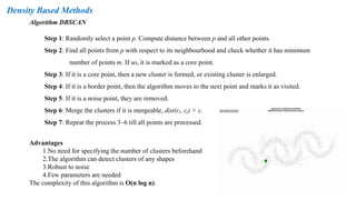
Algorithm DBSCAN
Step 1: Randomly select a point p. Compute distance between p and all other points.
Step 2: Find all points from p with respect to its neighbourhood and check whether it has minimum
number of points m. If so, it is marked as a core point.
Step 3: If it is a core point, then a new cluster is formed, or existing cluster is enlarged.
Step 4: If it is a border point, then the algorithm moves to the next point and marks it as visited.
Step 5: If it is a noise point, they are removed.
Step 6: Merge the clusters if it is mergeable, dist(cᵢ, cⱼ) < ε.
Step 7: Repeat the process 3–6 till all points are processed.
Advantages
1.No need for specifying the number of clusters beforehand
2.The algorithm can detect clusters of any shapes
3.Robust to noise
4.Few parameters are needed
The complexity of this algorithm is O(n log n).

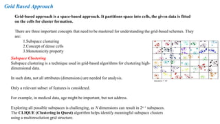
Grid-based approach is a space-based approach. It partitions space into cells, the given data is fitted
on the cells for cluster formation.
There are three important concepts that need to be mastered for understanding the grid-based schemes. They
are:
1.Subspace clustering
2.Concept of dense cells
3.Monotonicity property
Grid Based Approach
Subspace Clustering
Subspace clustering is a technique used in grid-based algorithms for clustering high-
dimensional data.
In such data, not all attributes (dimensions) are needed for analysis.
Only a relevant subset of features is considered.
For example, in medical data, age might be important, but not address.
Exploring all possible subspaces is challenging, as N dimensions can result in 2ⁿ⁻¹ subspaces.
The CLIQUE (Clustering in Quest) algorithm helps identify meaningful subspace clusters
using a multiresolution grid structure.

Concept of Dense Cells
CLIQUE partitions each dimension into several overlapping intervals and intervals it into cells.
Then, the algorithm determines whether the cell is dense or sparse.
The cell is considered dense if it exceeds a threshold value, say τ.
Density is defined as the ratio of number of points and volume of the region.
In one pass, the algorithm finds the number of cells, number of points, etc. and then combines the dense cells.
For that, the algorithm uses the contiguous intervals and a set of dense cells.
Algorithm Dense Cells
Step 1: Define a set of grid points and assign the given data points on the grid.
Step 2: Determine the dense and sparse cells. If the number of points in a cell exceeds the threshold
value τ, the cell is categorized as dense cell. Sparse cells are removed from the list.
Step 3: Merge the dense cells if they are adjacent.
Step 4: Form a list of grid cells for every subspace as output.
Grid Based Approach

Grid Based Approach
Monotonicity property
CLIQUE uses anti-monotonicity property or apriori property of the famous apriori algorithm.
It means that all the subsets of a frequent item should be frequent.
Similarly, if the subset is infrequent, then all its supersets are infrequent as well.
Based on the apriori property, one can conclude that a k-dimensional cell has r points if and only if every
(k−1) dimensional projections of this cell have atleast r points.
So like association rule mining that uses apriori rule, the candidate dense cells are generated for higher
dimensions.
Advantages of CLIQUE
1.Insensitive to input order of objects
2.No assumptions of underlying data distributions
3.Finds subspace of higher dimensions such that high-density clusters exist in those subspaces
Disadvantage
The disadvantage of CLIQUE is that tuning of grid parameters, such as grid size, and finding optimal threshold
for finding whether the cell is dense or not is a challenge.

Algorithm CLIQUE
Grid Based Approach
Stage 1:
1.Step 1: Identify the dense cells.
2.Step 2: Merge dense cells c1 and c2 if they share the same interval.
3.Step 3: Generate Apriori rule to generate (k+1)th cells for higher dimensions. Check whether the
number of points crosses the threshold. Repeat until no new dense cells are generated.
Stage 2:
1.Step 1: Merge dense cells into clusters in each subspace using maximal regions (hyperrectangle
covering all dense cells).
2.Step 2: Maximal regions cover all dense cells to form clusters.
*Note: Merging starts from dimension 2 and continues until the n-dimension.*

Clustering Algorithms - Kmeans,Min ALgorithm

More Related Content

More from Sharmila Chidaravalli (10)

Recently uploaded (20)

Clustering Algorithms - Kmeans,Min ALgorithm