SlideShare a Scribd company logo
Kernel Methods in Computer Vision

    Christoph Lampert                Matthew Blaschko

  Max Planck Institute for           MPI Tübingen and
  Biological Cybernetics, Tübingen   University of Oxford


                          June 20, 2009
Overview...

 14:00 – 15:00   Introduction to Kernel Classifiers

 15:20 – 15:50   Selecting and Combining Kernels

 15:50 – 16:20   Other Kernel Methods

 16:40 – 17:40   Learning with Structured Outputs


 Slides and Additional Material (soon)

 http://www.christoph-lampert.de


                             also watch out for
Introduction to Kernel Classifiers
Linear Classification

 Separates these two sample sets.


             height


                              width
Linear Classification

 Separates these two sample sets.


             height


                              width

                      Linear Classification
Linear Regression

 Find a function that interpolates data points.


               1.2


               1.0


               0.8


               0.6


               0.4


               0.2


               0.0
                 0.0    0.2    0.4     0.6    0.8   1.0
Linear Regression

 Find a function that interpolates data points.


               1.2


               1.0


               0.8


               0.6


               0.4


               0.2


               0.0
                 0.0    0.2    0.4     0.6    0.8   1.0


               Least Squares Regression
Linear Dimensionality Reduction

Reduce the dimensionality of a dataset while preserving its structure.

               4


               3


               2


               1


               0


               -1


               -2


               -3


               -4
                 -3   -2    -1     0     1      2     3


          Principal Component Analysis
Linear Techniques


Three different elementary tasks:
   classification,
   regression,
   dimensionality reduction.

In each case, linear techniques are very successful.
Linear Techniques


Linear techniques...

     often work well,
         most natural functions are smooth,
         smooth function can be approximated, at least locally, by
         linear functions.

     are fast and easy to solve
         elementary maths, even closed form solutions
         typically involve only matrix operation

     are intuitive
         solution can be visualized geometrically,
         solution corresponds to common sense.
Example: Maximum Margin Classification

Notation:
    data points X = {x1 , . . . , xn }, xi ∈ Rd ,
    class labels Y = {y1 , . . . , yn }, yi ∈ {+1, −1}.
     linear (decision) function f : Rd → R,
     decide classes based on sign f : Rd → {−1, 1}.

     parameterize

         f (x) = a 1 x 1 + a 2 x 2 + . . . a n x n + a 0
               ≡ w, x + b             with w = (a 1 , . . . , a n ), b = a 0 .

      . , . is the scalar product is Rd .
     f is uniquely determined by w ∈ Rd and b ∈ R,
     but we usually ignore b and only study w
          b can be absorbed into w. Set w = (w, b), x = (x, 1).
Example: Maximum Margin Classification

Given X = {x1 , . . . , xn }, Y = {y1 , . . . , yn }.


            2.0


            1.0


            0.0

             −1.0          0.0          1.0             2.0   3.0
Example: Maximum Margin Classification

Given X = {x1 , . . . , xn }, Y = {y1 , . . . , yn }. Any w partitions the
data space into two half-spaces, i.e. defines a classifier.


           2.0                   f (x) > 0

                                                    f (x) < 0
           1.0       w


           0.0

            −1.0          0.0         1.0         2.0         3.0
                         “What’s the best w?”
Example: Maximum Margin Classification


Given X = {x1 , . . . , xn }, Y = {y1 , . . . , yn }. What’s the best w?

  2.0                                   2.0


  1.0                                   1.0


  0.0                                   0.0

   −1.0    0.0     1.0     2.0    3.0   −1.0    0.0     1.0     2.0    3.0

Not these, since they misclassify many examples.

Criterion 1: Enforce sign w, xi = yi for i = 1, . . . , n.
Example: Maximum Margin Classification


Given X = {x1 , . . . , xn }, Y = {y1 , . . . , yn }. What’s the best w?

  2.0                                   2.0


  1.0                                   1.0


  0.0                                   0.0

   −1.0    0.0     1.0     2.0    3.0   −1.0    0.0     1.0     2.0    3.0

Better not these, since they would be “risky” for future samples.

Criterion 2: Try to ensure sign w, x = y for future (x, y) as well.
Example: Maximum Margin Classification

Given X = {x1 , . . . , xn }, Y = {y1 , . . . , yn }. Assume that future
samples are similar to current ones. What’s the best w?

  2.0

                         γ         γ
  1.0


  0.0

  −1.0     0.0     1.0       2.0       3.0

Maximize “stability”: use w such that we can maximally perturb the
input samples without introducing misclassifications.
Example: Maximum Margin Classification

Given X = {x1 , . . . , xn }, Y = {y1 , . . . , yn }. Assume that future
samples are similar to current ones. What’s the best w?

  2.0                                        2.0
                                                                        n
                                                                    rgi
                                                                  ma ion
                         γ         γ                            γ reg
  1.0                                        1.0


  0.0                                        0.0

  −1.0     0.0     1.0       2.0       3.0   −1.0   0.0   1.0    2.0        3.0

Maximize “stability”: use w such that we can maximally perturb the
input samples without introducing misclassifications.

Central quantity:
                                                                   w
    margin(x) = distance of x to decision hyperplane =             w
                                                                       ,x
Example: Maximum Margin Classification


Maximum-margin solution is determined by a maximization problem:

                   max        γ
                 w∈Rd ,γ∈R+


subject to

                sign w, xi = yi     for i = 1, . . . n.
                  w
                    , xi      ≥γ   for i = 1, . . . n.
                  w


Classify new samples using f (x) = w, x .
Example: Maximum Margin Classification


Maximum-margin solution is determined by a maximization problem:

                   max    γ
                w∈Rd , w =1
                   γ∈R


subject to

                  yi w, xi ≥ γ     for i = 1, . . . n.


Classify new samples using f (x) = w, x .
Example: Maximum Margin Classification


We can rewrite this as a minimization problem:
                                 2
                     mind
                             w
                     w∈R


subject to

                 yi w, xi ≥ 1        for i = 1, . . . n.


Classify new samples using f (x) = w, x .
Example: Maximum Margin Classification


From the view of optimization theory
                                  2
                      mind
                              w
                      w∈R


subject to

                  yi w, xi ≥ 1        for i = 1, . . . n

is rather easy:
      The objective function is differentiable and convex.
      The constraints are all linear.
We can find the globally optimal w in O(n 3 ) (or faster).
Linear Separability

 What is the best w for this dataset?


              height


                               width
Linear Separability

 What is the best w for this dataset?


              height


                               width
 Not this.
Linear Separability

 What is the best w for this dataset?


              height


                               width
 Not this.
Linear Separability

 What is the best w for this dataset?


              height


                               width
 Not this.
Linear Separability

 What is the best w for this dataset?


              height


                               width
 Not this.
Linear Separability

  The problem
           2
  min w


                                         ?
  w∈Rd


                         height
  subject to

    yi w, xi ≥ 1

  has no solution.
  The constraints con-
  tradict each other!                  width

 We cannot find a maximum-margin hyperplane here, because there
 is none. To fix this, we must allow hyperplanes that make mistakes.
Linear Separability

 What is the best w for this dataset?


              height


                               width
Linear Separability

 What is the best w for this dataset?


                                                          n
                                                     a tio
                                                ol
                                             vi
                                        in
              height


                                    a rg
                                  m
                                  ξ


                               width
 Possibly this one, even though one sample is misclassified.
Linear Separability

 What is the best w for this dataset?


              height


                               width
Linear Separability

 What is the best w for this dataset?


                                         small
                                            in
                                        marg
                                    ve r y
              height


                               width
 Maybe not this one, even though all points are classified correctly.
Linear Separability

 What is the best w for this dataset?


                                                      n
                                                   tio
              height


                                                 a
                                            ol
                                       vi
                                  in
                              a rg
                             m
                         ξ

                                width
 Trade-off: large margin vs. few mistakes on training set
Solving for Soft-Margin Solution

 Mathematically, we formulate the trade-off by slack-variables ξi :
                                          n
                                 2
                  min        w       +C         ξi
               w∈R ,ξi ∈R+
                  d
                                          i=1


 subject to
                 yi w, xi ≥ 1 − ξi              for i = 1, . . . n.

     We can fulfill every constraint by choosing ξi large enough.
     The larger ξi , the larger the objective (that we try to minimize).
     C is a regularization/trade-off parameter:
          small C → constraints are easily ignored
          large C → constraints are hard to ignore
          C = ∞ → hard margin case → no training error
     Note: The problem is still convex and efficiently solvable.
Linear Separability

 So, what is the best soft-margin w for this dataset?

                                       y


                                                        x


 None. We need something non-linear!
Non-Linear Classification: Stacking

 Idea 1) Use classifier output as input to other (linear) classifiers:

                fi=<wi,x>

                                       σ(f5(x'))


                 σ(f1(x))   σ(f2(x))           σ(f3(x))   σ(f4(x))


 Multilayer Perceptron (Artificial Neural Network) or Boosting
 ⇒ decisions depend non-linearly on x and wj .
Non-linearity: Data Preprocessing

 Idea 2) Preprocess the data:
                                                 y


  This dataset is not
  (well) linearly separable:                             x


                         θ

  This one is:
                                                     r


 In fact, both are the same dataset!
 Top: Cartesian coordinates. Bottom: polar coordinates
Non-linearity: Data Preprocessing


                                                     y


  Non-linear separation                                        x


                       θ
  Linear
  separation                                          r


 Linear classifier in polar space; acts non-linearly in Cartesian space.
Generalized Linear Classifier

     Given X = {x1 , . . . , xn }, Y = {y1 , . . . , yn }.
     Given any (non-linear) feature map ϕ : Rk → Rm .
     Solve the minimization for ϕ(x1 ), . . . , ϕ(xn ) instead of
     x1 , . . . , xn :
                                              n
                                     2
                      min        w       +C         ξi
                   w∈R ,ξi ∈R+
                      m
                                              i=1


     subject to
                  yi w, ϕ(xi ) ≥ 1 − ξi             for i = 1, . . . n.

     The weight vector w now comes from the target space Rm .
     Distances/angles are measure by the scalar product . , . in Rm .

     Classifier f (x) = w, ϕ(x) is linear in w, but non-linear in x.
Example Feature Mappings


    Polar coordinates:
                                                 √
                                 x                  x 2 + y2
                              ϕ:   →
                                 y                 ∠(x, y)

    d-th degree polynomials:
                                                 2            2            d            d
     ϕ : x1 , . . . , xn → 1, x1 , . . . , xn , x1 , . . . , xn , . . . , x1 , . . . , xn

    Distance map:

                       ϕ:x→            x − pi , . . . , x − pN

    for a set of N prototype vectors pi , i = 1, . . . , N .
Is this enough?

 In this example, changing the coordinates did help.
 Does this trick always work?
                                                 y

                θ
                                                       x
                                   r   ↔
Is this enough?

 In this example, changing the coordinates did help.
 Does this trick always work?
                                                    y

                 θ
                                                         x
                                    r   ↔


 Answer: In a way, yes!
 Lemma
 Let (xi )i=1,...,n with xi = xj for i = j. Let ϕ : Rk → Rm be a feature
 map. If the set ϕ(xi )i=1,...,n is linearly independent, then the points
 ϕ(xi )i=1,...,n are linearly separable.

 Lemma
 If we choose m > n large enough, we can always find a map ϕ.
Is this enough?


 Caveat: We can separate any set, not just one with “reasonable” yi :


 There is a fixed feature map ϕ : R2 → R20001 such that – no matter
 how we label them – there is always a hyperplane classifier that has
 zero training error.
Is this enough?


 Caveat: We can separate any set, not just one with “reasonable” yi :


 There is a fixed feature map ϕ : R2 → R20001 such that – no matter
 how we label them – there is always a hyperplane classifier that has
 0 training error.
Representer Theorem

Solve the soft-margin minimization for ϕ(x1 ), . . . , ϕ(xn ) ∈ Rm :
                                         n
                                2
                 min        w       +C         ξi                         (1)
             w∈Rm ,ξi ∈R+
                                         i=1

subject to

                  yi w, ϕ(xi ) ≥ 1 − ξi             for i = 1, . . . n.
For large m, won’t solving for w ∈ Rm become impossible?
Representer Theorem

Solve the soft-margin minimization for ϕ(x1 ), . . . , ϕ(xn ) ∈ Rm :
                                              n
                                    2
                   min          w       +C         ξi                           (1)
             w∈Rm ,ξi ∈R+
                                             i=1

subject to

                    yi w, ϕ(xi ) ≥ 1 − ξi               for i = 1, . . . n.
For large m, won’t solving for w ∈ Rm become impossible?                      No!

Theorem (Representer Theorem)
The minimizing solution w to problem (1) can always be written as
               n
        w=          αj ϕ(xj )           for coefficients α1 , . . . , αn ∈ R.
              j=1
Kernel Trick


 The representer theorem allows us to rewrite the optimization:
                                            n
                                   2
                 min         w         +C         ξi
              w∈R ,ξi ∈R+
                 m
                                            i=1


 subject to

                  yi w, ϕ(xi ) ≥ 1 − ξi                for i = 1, . . . n.
                n
 Insert w =     j=1   αj ϕ(xj ):
Kernel Trick


 We can minimize over αi instead of w:
                           n                         n
                                            2
           min                  αj ϕ(xj )       +C         ξi
        αi ∈R,ξi ∈R+
                          j=1                        i=1


 subject to
                   n
              yi         αj ϕ(xj ), ϕ(xi ) ≥ 1 − ξi             for i = 1, . . . n.
                   j=1
Kernel Trick


          2
 Use w        = w, w :
                   n                                  n
      min                 αj αk ϕ(xj ), ϕ(xk ) + C         ξi
   αi ∈R,ξi ∈R+
                  j,k=1                              i=1


 subject to
                          n
                    yi         αj ϕ(xj ), ϕ(xi ) ≥ 1 − ξi       for i = 1, . . . n.
                         j=1


 Note: ϕ only occurs in ϕ(.), ϕ(.) pairs.
Kernel Trick


 Set ϕ(x), ϕ(x ) =: k(x, x ), called kernel function.
                      n                              n
         min                 αj αk k(xj , xk ) + C         ξi
      αi ∈R,ξi ∈R+
                     j,k=1                           i=1


 subject to
                             n
                       yi         αj k(xj , xi ) ≥ 1 − ξi       for i = 1, . . . n.
                            j=1

 The maximum-margin classifier in this form with a kernel function is
 often called Support-Vector Machine (SVM).
Why use k(x, x ) instead of ϕ(x), ϕ(x ) ?

1) Speed:
    We might find an expression for k(xi , xj ) that is faster to
    calculate than forming ϕ(xi ) and then ϕ(xi ), ϕ(xj ) .

     Example: 2nd-order polynomial kernel (here for x ∈ R1 ):
                                 √
                     ϕ : x → (1, 2x, x 2 ) ∈ R3

                                  √                √
              ϕ(xi ), ϕ(xj ) = (1, 2xi , xi2 ), (1, 2xj , xj2 )
                              = 1 + 2xi xj + xi2 xj2

     But equivalently (and faster) we can calculate without ϕ:

                  k(xi , xj ) : = (1 + xi xj )2
                              = 1 + 2xi xj + xi2 xj2
Why use k(x, x ) instead of ϕ(x), ϕ(x ) ?


2) Flexibility:
     There are kernel functions k(xi , xj ), for which we know that a
     feature transformation ϕ exists, but we don’t know what ϕ is.
Why use k(x, x ) instead of ϕ(x), ϕ(x ) ?


2) Flexibility:
     There are kernel functions k(xi , xj ), for which we know that a
     feature transformation ϕ exists, but we don’t know what ϕ is.
     How that???


Theorem
Let k : X × X → R be a positive definite kernel function. Then
there exists a Hilbert Space H and a mapping ϕ : X → H such
that

                          k(x, x ) = ϕ(x), ϕ(x )   H


where . , .   H   is the inner product in H.
Positive Definite Kernel Function

Definition (Positive Definite Kernel Function)
Let X be a non-empty set. A function k : X × X → R is called
positive definite kernel function, iff
    k is symmetric, i.e. k(x, x ) = k(x , x) for all x, x ∈ X .
    For any set of points x1 , . . . , xn ∈ X , the matrix

                             Kij = (k(xi , xj ))i,j

     is positive (semi-)definite, i.e. for all vectors t ∈ Rn :
                                n
                                       ti Kij tj ≥ 0.
                               i,j=1


Note: Instead of “positive definite kernel function”, we will often
just say “kernel”.
Hilbert Spaces


Definition (Hilbert Space)
A Hilbert Space H is a vector space H with an inner product
 . , . H , e.g. a mapping

                         .,. H : H × H → R
which is
    symmetric: v, v H = v , v H for all v, v ∈ H ,
    positive definite: v, v H ≥ 0 for all v ∈ H ,
              where v, v H = 0 only for v = 0 ∈ H .
    bilinear: av, v H = a v, v H for v ∈ H , a ∈ R
               v + v , v H = v, v H + v , v H

We can treat a Hilbert space like some Rn , if we only use concepts
like vectors, angles, distances. Note: dim H = ∞ is possible!
Kernels for Arbitrary Sets

 Theorem
 Let k : X × X → R be a positive definite kernel function. Then
 there exists a Hilbert Space H and a mapping ϕ : X → H such
 that

                           k(x, x ) = ϕ(x), ϕ(x )   H


 where . , .   H   is the inner product in H.


 Translation
 Take any set X and any function k : X × X → R.
 If k is a positive definite kernel, then we can use k to learn a (soft)
 maximum-margin classifier for the elements in X !

 Note: X can be any set, e.g. X = { all images }.
How to Check if a Function is a Kernel


 Problem:
     Checking if a given k : X × X → R fulfills the conditions for a
     kernel is difficult:
     We need to prove or disprove
                             n
                                   ti k(xi , xj )tj ≥ 0.
                           i,j=1

     for any set x1 , . . . , xn ∈ X and any t ∈ Rn for any n ∈ N.
 Workaround:
     It is easy to construct functions k that are positive definite
     kernels.
Constructing Kernels


1) We can construct kernels from scratch:
    For any ϕ : X → Rm , k(x, x ) = ϕ(x), ϕ(x ) Rm is a kernel.
    If d : X × X → R is a distance function, i.e.
       • d(x, x ) ≥ 0 for all x, x ∈ X ,
       • d(x, x ) = 0 only for x = x ,
       • d(x, x ) = d(x , x) for all x, x ∈ X ,
       • d(x, x ) ≤ d(x, x ) + d(x , x ) for all x, x , x ∈ X ,
     then k(x, x ) := exp(−d(x, x )) is a kernel.

2) We can construct kernels from other kernels:
    if k is a kernel and α > 0, then αk and k + α are kernels.
    if k1 , k2 are kernels, then k1 + k2 and k1 · k2 are kernels.
Constructing Kernels


Examples for kernels for X = Rd :
    any linear combination j αj kj with αj ≥ 0,
    polynomial kernels k(x, x ) = (1 + x, x )m , m > 0
                                        x−x     2
     Gaussian or RBF k(x, x ) = exp −    2σ 2
                                                    with σ > 0,
Constructing Kernels


Examples for kernels for X = Rd :
    any linear combination j αj kj with αj ≥ 0,
    polynomial kernels k(x, x ) = (1 + x, x )m , m > 0
                                         x−x     2
     Gaussian or RBF k(x, x ) = exp −     2σ 2
                                                     with σ > 0,
Examples for kernels for other X :
    k(h, h ) = n min(hi , hi ) for n-bin histograms h, h .
                 i=1
    k(p, p ) = exp(−KL(p, p )) with KL the symmetrized
    KL-divergence between positive probability distributions.
    k(s, s ) = exp(−D(s, s )) for strings s, s and D = edit distance
Examples for functions X × X → R that are not kernels:
     tanh (κ x, x + θ) (matrix Kij can have negative eigenvalues)
Kernels in Computer Vision


X = { images }, treat feature extraction as part of kernel definition

     OCR/handwriting recognition
         resize image, normalize brightness/contrast/rotation/skew
         polynomial kernel k(x, x ) = (1 + x, x )d , d > 0
         [DeCoste, Schölkopf. ML2002]

     Pedestrian detection
         resize image, calculate local intensity gradient directions
         local thresholding + linear kernel [Dalal, Triggs. CVPR 2005]
         or
         local L1 -normalization + histogram intersection kernel
         [Maji, Berg, Malik. CVPR 2008]
Kernels in Computer Vision

X = { images }, treat feature extraction as part of kernel definition
   object category recognition
         extract local image descriptors, e.g. SIFT
         calculate multi-level pyramid histograms h l,k (x)
         pyramid match kernel [Grauman, Darrell. ICCV 2005]
                                  L            2l−1
                                           l
                kPMK (x, x ) =         2              min h l,k (x), h l,k (x )
                                 l=1           k=1

     scene/object category recognition
         extract local image descriptors, e.g. SIFT
         quantize descriptors into bag-of-words histograms
         χ2 -kernel [Puzicha, Buhmann, Rubner, Tomasi. ICCV1999]

            kχ2 (h, h ) = exp −γχ2 (h, h )                   for γ > 0
                            K
                               (hk − hk )2
             χ2 (h, h ) =
                            k=1 hk + hk
Summary

Linear methods are popular and well understood
    classification, regression, dimensionality reduction, ...

Kernels are at the same time...
 1) Similarity measure between (arbitrary) objects,
 2) Scalar products in a (hidden) vector space.

Kernelization can make linear techniques more powerful
    implicit preprocessing, non-linear in the original data.
    still linear in some feature space ⇒ still intuitive/interpretable

Kernels can be defined over arbitrary inputs, e.g. images
    unified framework for all preprocessing steps
    different features, normalization, etc., becomes kernel choices
What did we not see?

We have skipped the largest part of theory on kernel methods:
    Optimization
         Dualization
         Algorithms to train SVMs
    Kernel Design
         Systematic methods to construct data-dependent kernels.
    Statistical Interpretations
         What do we assume about samples?
         What performance can we expect?
    Generalization Bounds
         The test error of a (kernelized) linear classifier can be
         controlled using its modelling error and its training error.

    “Support Vectors”
This and much more in standard references.
Selecting and Combining Kernels
Selecting From Multiple Kernels

Typically, one has many different kernels to choose from:
    different functional forms
         linear, polynomial, RBF, . . .
     different parameters
         polynomial degree, Gaussian bandwidth, . . .
Selecting From Multiple Kernels

Typically, one has many different kernels to choose from:
    different functional forms
         linear, polynomial, RBF, . . .
     different parameters
         polynomial degree, Gaussian bandwidth, . . .
Different image features give rise to different kernels
    Color histograms,
    SIFT bag-of-words,
    HOG,
    Pyramid match,
    Spatial pyramids, . . .

How to choose?
   Ideally, based on the kernels’ performance on task at hand:
         estimate by cross-validation or validation set error
     Classically part of “Model Selection”.
Kernel Parameter Selection


Note: Model Selection makes a difference!
    Action Classification, KTH dataset

       Method                                        Accuracy
       Dollár et al. VS-PETS 2005: ”SVM classifier“      80.66
       Nowozin et al., ICCV 2007: ”baseline RBF“        85.19
     identical features, same kernel function
     difference: Nowozin used cross-validation for model selection
     (bandwidth and C )

Note: there is no overfitting involved here. Model selection is fully
automatic and uses only training data.
Kernel Parameter Selection

Rule of thumb for kernel parameters
     For kernels based on the exponential function
                                        1
                        k(x, x ) = exp(− X (x, x ))
                                        γ
     with any X , set

                        γ ≈ meani,j=1,...,n X (xi , xj ).

     Sometimes better: use only X (xi , xj ) with yi = yj .
     In general, if there are several classes, then the kernel matrix :

                               Kij = k(xi , xj )

     should have a block structure w.r.t. the classes.
1.0                                                                               1.0
                                                 0                                0.9    0                                        0                                 0.9
                                                                                                                          2.4
 1.0                     y                                                        0.8                                                                               0.8
                                                10                                      10                                1.6
                                                                                                                                 10
                                                                                  0.7                                                                               0.7
 0.5
                                          x
                                                20                                0.6
                                                                                        20
                                                                                                                          0.8
                                                                                                                                 20                                 0.6

                                                                                  0.5                                                                               0.5
 0.0                                                                                                                      0.0

                                                30                                0.4   30                                       30                                 0.4
                                                                                                                          −0.8
−0.5                                                                              0.3                                                                               0.3

                                                40                                0.2   40                                −1.6   40                                 0.2
−1.0                                                                              0.1                                     −2.4                                      0.1

         −2.0   −1.0   0.0    1.0        2.0         0   10   20   30   40   50   0.0        0   10   20   30   40   50               0   10    20   30   40   50   0.0


          two moons                                  label “kernel”                                   linear                     RBF: γ = 0.001
                                          1.0                                     1.0                                      1.0                                      1.0
 0                                        0.9
                                                 0                                0.9
                                                                                         0                                 0.9
                                                                                                                                  0                                 0.9

                                          0.8                                     0.8                                      0.8                                      0.8
10                                              10                                      10                                       10
                                          0.7                                     0.7                                      0.7                                      0.7


20                                        0.6
                                                20                                0.6
                                                                                        20                                 0.6
                                                                                                                                 20                                 0.6

                                          0.5                                     0.5                                      0.5                                      0.5

30                                        0.4   30                                0.4   30                                 0.4   30                                 0.4

                                          0.3                                     0.3                                      0.3                                      0.3

40                                        0.2   40                                0.2   40                                 0.2   40                                 0.2

                                          0.1                                     0.1                                      0.1                                      0.1

     0     10    20    30    40     50    0.0        0   10   20   30   40   50   0.0        0   10   20   30   40   50    0.0        0   10    20   30   40   50   0.0


            γ = 0.01                                      γ = 0.1                                     γ=1                                      γ = 10
                                          1.0                                     1.0
 0                                        0.9
                                                 0                                0.9

                                          0.8                                     0.8
10                                              10
                                          0.7                                     0.7


20                                        0.6
                                                20                                0.6

                                          0.5                                     0.5

30                                        0.4   30                                0.4

                                          0.3                                     0.3

40                                        0.2   40                                0.2

                                          0.1                                     0.1

     0     10    20    30    40     50    0.0        0   10   20   30   40   50   0.0


                γ = 100                                  γ = 1000
1.0                                                                               1.0
                                                 0                                0.9    0                                        0                                 0.9
                                                                                                                          2.4
 1.0                     y                                                        0.8                                                                               0.8
                                                10                                      10                                1.6
                                                                                                                                 10
                                                                                  0.7                                                                               0.7
 0.5
                                          x
                                                20                                0.6
                                                                                        20
                                                                                                                          0.8
                                                                                                                                 20                                 0.6

                                                                                  0.5                                                                               0.5
 0.0                                                                                                                      0.0

                                                30                                0.4   30                                       30                                 0.4
                                                                                                                          −0.8
−0.5                                                                              0.3                                                                               0.3

                                                40                                0.2   40                                −1.6   40                                 0.2
−1.0                                                                              0.1                                     −2.4                                      0.1

         −2.0   −1.0   0.0    1.0        2.0         0   10   20   30   40   50   0.0        0   10   20   30   40   50               0   10    20   30   40   50   0.0


          two moons                                  label “kernel”                                   linear                     RBF: γ = 0.001
                                          1.0                                     1.0                                      1.0                                      1.0
 0                                        0.9
                                                 0                                0.9
                                                                                         0                                 0.9
                                                                                                                                  0                                 0.9

                                          0.8                                     0.8                                      0.8                                      0.8
10                                              10                                      10                                       10
                                          0.7                                     0.7                                      0.7                                      0.7


20                                        0.6
                                                20                                0.6
                                                                                        20                                 0.6
                                                                                                                                 20                                 0.6

                                          0.5                                     0.5                                      0.5                                      0.5

30                                        0.4   30                                0.4   30                                 0.4   30                                 0.4

                                          0.3                                     0.3                                      0.3                                      0.3

40                                        0.2   40                                0.2   40                                 0.2   40                                 0.2

                                          0.1                                     0.1                                      0.1                                      0.1

     0     10    20    30    40     50    0.0        0   10   20   30   40   50   0.0        0   10   20   30   40   50    0.0        0   10    20   30   40   50   0.0


            γ = 0.01                                      γ = 0.1                                     γ=1                                      γ = 10
                                          1.0                                     1.0                                      1.0
 0                                        0.9
                                                 0                                0.9
                                                                                         0                                 0.9

                                          0.8                                     0.8                                      0.8
10                                              10                                      10
                                          0.7                                     0.7                                      0.7


20                                        0.6
                                                20                                0.6
                                                                                        20                                 0.6

                                          0.5                                     0.5                                      0.5

30                                        0.4   30                                0.4   30                                 0.4

                                          0.3                                     0.3                                      0.3

40                                        0.2   40                                0.2   40                                 0.2

                                          0.1                                     0.1                                      0.1

     0     10    20    30    40     50    0.0        0   10   20   30   40   50   0.0        0   10   20   30   40   50    0.0


                γ = 100                                  γ = 1000                               γ = 0.6
                                                                                             rule of thumb
1.0                                                                               1.0
                                                 0                                0.9    0                                        0                                 0.9
                                                                                                                          2.4
 1.0                     y                                                        0.8                                                                               0.8
                                                10                                      10                                1.6
                                                                                                                                 10
                                                                                  0.7                                                                               0.7
 0.5
                                          x
                                                20                                0.6
                                                                                        20
                                                                                                                          0.8
                                                                                                                                 20                                 0.6

                                                                                  0.5                                                                               0.5
 0.0                                                                                                                      0.0

                                                30                                0.4   30                                       30                                 0.4
                                                                                                                          −0.8
−0.5                                                                              0.3                                                                               0.3

                                                40                                0.2   40                                −1.6   40                                 0.2
−1.0                                                                              0.1                                     −2.4                                      0.1

         −2.0   −1.0   0.0    1.0        2.0         0   10   20   30   40   50   0.0        0   10   20   30   40   50               0   10    20   30   40   50   0.0


          two moons                                  label “kernel”                                   linear                     RBF: γ = 0.001
                                          1.0                                     1.0                                      1.0                                      1.0
 0                                        0.9
                                                 0                                0.9
                                                                                         0                                 0.9
                                                                                                                                  0                                 0.9

                                          0.8                                     0.8                                      0.8                                      0.8
10                                              10                                      10                                       10
                                          0.7                                     0.7                                      0.7                                      0.7


20                                        0.6
                                                20                                0.6
                                                                                        20                                 0.6
                                                                                                                                 20                                 0.6

                                          0.5                                     0.5                                      0.5                                      0.5

30                                        0.4   30                                0.4   30                                 0.4   30                                 0.4

                                          0.3                                     0.3                                      0.3                                      0.3

40                                        0.2   40                                0.2   40                                 0.2   40                                 0.2

                                          0.1                                     0.1                                      0.1                                      0.1

     0     10    20    30    40     50    0.0        0   10   20   30   40   50   0.0        0   10   20   30   40   50    0.0        0   10    20   30   40   50   0.0


            γ = 0.01                                      γ = 0.1                                     γ=1                                      γ = 10
                                          1.0                                     1.0                                      1.0                                      1.0
 0                                        0.9
                                                 0                                0.9
                                                                                         0                                 0.9
                                                                                                                                  0                                 0.9

                                          0.8                                     0.8                                      0.8                                      0.8
10                                              10                                      10                                       10
                                          0.7                                     0.7                                      0.7                                      0.7


20                                        0.6
                                                20                                0.6
                                                                                        20                                 0.6
                                                                                                                                 20                                 0.6

                                          0.5                                     0.5                                      0.5                                      0.5

30                                        0.4   30                                0.4   30                                 0.4   30                                 0.4

                                          0.3                                     0.3                                      0.3                                      0.3

40                                        0.2   40                                0.2   40                                 0.2   40                                 0.2

                                          0.1                                     0.1                                      0.1                                      0.1

     0     10    20    30    40     50    0.0        0   10   20   30   40   50   0.0        0   10   20   30   40   50    0.0        0   10    20   30   40   50   0.0


                γ = 100                                  γ = 1000                               γ = 0.6                                    γ = 1.6
                                                                                             rule of thumb                                5-fold CV
Kernel Selection ↔ Kernel Combination

Is there a single best kernel at all?
     Kernels are typcally designed to capture one aspect of the data
         texture, color, edges, . . .
    Choosing one kernel means to select exactly one such aspect.
Kernel Selection ↔ Kernel Combination

Is there a single best kernel at all?
     Kernels are typcally designed to capture one aspect of the data
         texture, color, edges, . . .
    Choosing one kernel means to select exactly one such aspect.
    Combining aspects if often better than Selecting.
                      Method             Accuracy
                      Colour            60.9 ± 2.1
                      Shape             70.2 ± 1.3
                      Texture           63.7 ± 2.7
                      HOG               58.5 ± 4.5
                      HSV               61.3 ± 0.7
                      siftint           70.6 ± 1.6
                      siftbdy           59.4 ± 3.3
                      combination       85.2 ± 1.5
Mean accuracy on Oxford Flowers dataset [Gehler, Nowozin: ICCV2009]
Combining Two Kernels


For two kernels k1 , k2 :
     product k = k1 k2 is again a kernel
         Problem: very small kernel values suppress large ones

    average k = 1 (k1 + k2 ) is again a kernel
                2
         Problem: k1 , k2 on different scales. Re-scale first?
         convex combination kβ = (1 − β)k1 + βk2 with β ∈ [0, 1]

    Model selection: cross-validate over β ∈ {0, 0.1, . . . , 1}.
Combining Many Kernels

Multiple kernels: k1 ,. . . ,kK
    all convex combinations are kernels:
                    K                            K
               k=         βj kj   with βj ≥ 0,         β = 1.
                    j=1                          j=1

    Kernels can be “deactivated” by βj = 0.
    Combinatorial explosion forbids cross-validation over all
    combinations of βj
Proxy: instead of CV, maximize SVM-objective.
    Each combined kernel induces a feature space.
    In which of the feature spaces can we best
         explain the training data, and
         achieve a large margin between the classes?
Feature Space View of Kernel Combination

Each kernel kj induces
    a Hilbert Space Hj and a mapping ϕj : X → Hj .
                           β
The weighted kernel kj j := βj kj induces
    the same Hilbert Space Hj , but
                                    β
    a rescaled feature mapping ϕj j (x) :=                 βj ϕj (x).
                       β           β
     k βj (x, x ) ≡ ϕj j (x), ϕj j (x )      H   =     βj ϕj (x), βj ϕj (x )           H

                = βj ϕj (x), ϕj (x )         H   = βj k(x, x ).

                       ˆ
The linear combination k := K βj kj induces
                            j=1
    the product space H := ⊕K Hj , and
                            j=1
    the product mapping ϕ(x) := (ϕβ1 (x), . . . , ϕβn (x))t
                          ˆ       1                n
                                       K                                     K
  ˆ                                           β         β
  k(x, x ) ≡ ϕ(x), ϕ(x )
             ˆ     ˆ           H
                                   =         ϕj j (x), ϕj j (x   )   H   =         βj k(x, x )
                                       j=1                                   j=1
Feature Space View of Kernel Combination

Implicit representation of a dataset using two kernels:


     Kernel k1 , feature representation ϕ1 (x1 ), . . . , ϕ1 (xn ) ∈ H1


     Kernel k2 , feature representation ϕ2 (x1 ), . . . , ϕ2 (xn ) ∈ H2

Kernel Selection would most likely pick k2 .
For k = (1 − β)k1 + βk2 , top is β = 0, bottom is β = 1.
Feature Space View of Kernel Combination

                                   β = 0.00   margin = 0.0000
        5
            √
                1.00φ2 (xi )                                        H1 × H2

        4


        3


        2


        1


        0

                                                                    √
                                                                        0.00φ1 (xi )
       −1
        −1                     0      1        2         3      4                      5
Feature Space View of Kernel Combination

                                   β = 1.00   margin = 0.1000
        5
            √
                0.00φ2 (xi )                                        H1 × H2

        4


        3


        2


        1


        0

                                                                    √
                                                                        1.00φ1 (xi )
       −1
        −1                     0      1        2         3      4                      5
Feature Space View of Kernel Combination

                                   β = 0.99   margin = 0.2460
        5
            √
                0.01φ2 (xi )                                        H1 × H2

        4


        3


        2


        1


        0

                                                                    √
                                                                        0.99φ1 (xi )
       −1
        −1                     0      1        2         3      4                      5
Feature Space View of Kernel Combination

                                   β = 0.98   margin = 0.3278
        5
            √
                0.02φ2 (xi )                                        H1 × H2

        4


        3


        2


        1


        0

                                                                    √
                                                                        0.98φ1 (xi )
       −1
        −1                     0      1        2         3      4                      5
Feature Space View of Kernel Combination

                                   β = 0.97   margin = 0.3809
        5
            √
                0.03φ2 (xi )                                        H1 × H2

        4


        3


        2


        1


        0

                                                                    √
                                                                        0.97φ1 (xi )
       −1
        −1                     0      1        2         3      4                      5
Feature Space View of Kernel Combination

                                   β = 0.95   margin = 0.4515
        5
            √
                0.05φ2 (xi )                                        H1 × H2

        4


        3


        2


        1


        0

                                                                    √
                                                                        0.95φ1 (xi )
       −1
        −1                     0      1        2         3      4                      5
Feature Space View of Kernel Combination

                                   β = 0.90   margin = 0.5839
        5
            √
                0.10φ2 (xi )                                        H1 × H2

        4


        3


        2


        1


        0

                                                                    √
                                                                        0.90φ1 (xi )
       −1
        −1                     0      1        2         3      4                      5
Feature Space View of Kernel Combination

                                   β = 0.80   margin = 0.7194
        5
            √
                0.20φ2 (xi )                                        H1 × H2

        4


        3


        2


        1


        0

                                                                    √
                                                                        0.80φ1 (xi )
       −1
        −1                     0      1        2         3      4                      5
Feature Space View of Kernel Combination

                                   β = 0.70   margin = 0.7699
        5
            √
                0.30φ2 (xi )                                        H1 × H2

        4


        3


        2


        1


        0

                                                                    √
                                                                        0.70φ1 (xi )
       −1
        −1                     0      1        2         3      4                      5
Feature Space View of Kernel Combination

                                   β = 0.65   margin = 0.7770
        5
            √
                0.35φ2 (xi )                                        H1 × H2

        4


        3


        2


        1


        0

                                                                    √
                                                                        0.65φ1 (xi )
       −1
        −1                     0      1        2         3      4                      5
Feature Space View of Kernel Combination

                                   β = 0.60   margin = 0.7751
        5
            √
                0.40φ2 (xi )                                        H1 × H2

        4


        3


        2


        1


        0

                                                                    √
                                                                        0.60φ1 (xi )
       −1
        −1                     0      1        2         3      4                      5
Feature Space View of Kernel Combination

                                   β = 0.50   margin = 0.7566
        5
            √
                0.50φ2 (xi )                                        H1 × H2

        4


        3


        2


        1


        0

                                                                    √
                                                                        0.50φ1 (xi )
       −1
        −1                     0      1        2         3      4                      5
Feature Space View of Kernel Combination

                                   β = 0.40   margin = 0.7365
        5
            √
                0.60φ2 (xi )                                        H1 × H2

        4


        3


        2


        1


        0

                                                                    √
                                                                        0.40φ1 (xi )
       −1
        −1                     0      1        2         3      4                      5
Feature Space View of Kernel Combination

                                   β = 0.30   margin = 0.7073
        5
            √
                0.70φ2 (xi )                                        H1 × H2

        4


        3


        2


        1


        0

                                                                    √
                                                                        0.30φ1 (xi )
       −1
        −1                     0      1        2         3      4                      5
Feature Space View of Kernel Combination

                                   β = 0.20   margin = 0.6363
        5
            √
                0.80φ2 (xi )                                        H1 × H2

        4


        3


        2


        1


        0

                                                                    √
                                                                        0.20φ1 (xi )
       −1
        −1                     0      1        2         3      4                      5
Feature Space View of Kernel Combination

                                   β = 0.10   margin = 0.4928
        5
            √
                0.90φ2 (xi )                                        H1 × H2

        4


        3


        2


        1


        0

                                                                    √
                                                                        0.10φ1 (xi )
       −1
        −1                     0      1        2         3      4                      5
Feature Space View of Kernel Combination

                                   β = 0.03   margin = 0.2870
        5
            √
                0.97φ2 (xi )                                        H1 × H2

        4


        3


        2


        1


        0

                                                                    √
                                                                        0.03φ1 (xi )
       −1
        −1                     0      1        2         3      4                      5
Feature Space View of Kernel Combination

                                   β = 0.02   margin = 0.2363
        5
            √
                0.98φ2 (xi )                                        H1 × H2

        4


        3


        2


        1


        0

                                                                    √
                                                                        0.02φ1 (xi )
       −1
        −1                     0      1        2         3      4                      5
Feature Space View of Kernel Combination

                                   β = 0.01   margin = 0.1686
        5
            √
                0.99φ2 (xi )                                        H1 × H2

        4


        3


        2


        1


        0

                                                                    √
                                                                        0.01φ1 (xi )
       −1
        −1                     0      1        2         3      4                      5
Feature Space View of Kernel Combination

                                   β = 0.00   margin = 0.0000
        5
            √
                1.00φ2 (xi )                                        H1 × H2

        4


        3


        2


        1


        0

                                                                    √
                                                                        0.00φ1 (xi )
       −1
        −1                     0      1        2         3      4                      5
Multiple Kernel Learning


 Can we calculate coefficients βj that realize the largest margin?
     Analyze: how does the margin depend on βj ?
     Remember standard SVM (here without slack variables):
                                    2
                          min w     H
                          w∈H


     subject to

                    yi w, xi   H   ≥1   for i = 1, . . . n.

     H and ϕ were induced by kernel k.
     New samples are classified by f (x) = w, x      H.
Multiple Kernel Learning

     Insert
                                               K
                            k(x, x ) =               βj kj (x, x )           (2)
                                               j=1

     with
            Hilbert space H = ⊕j√ j ,
                                H                   √
            feature map ϕ(x) = ( β1 ϕ1 (x), . . . , βK ϕK (x))t ,
            weight vector w = (w1 , . . . , wK )t .
     such that
                                   2                    2
                             w     H   =           wj   Hj                   (3)
                                           j

                       w, ϕ(xi )   H   =             βj wj , ϕj (xi )   Hj   (4)
                                           j
Multiple Kernel Learning

     For fixed βj , the largest margin hyperplane is given by
                                  2
           min               wj   Hj
           wj ∈Hj
                     j

     subject to

              yi             βj wj , ϕj (xi )      Hj   ≥1      for i = 1, . . . n.
                     j

                                                         0
     Renaming vj =            βj wj (and defining         0
                                                             = 0):
                              1        2
              min                vj    Hj
              vj ∈Hj
                         j    βj

     subject to
                    yi        vj , ϕj (xi )   Hj   ≥1        for i = 1, . . . n.
                         j
Multiple Kernel Learning


     Therefore, best hyperplane for variable βj is given by:
                                                 1       2
                                    min             vj   Hj                (5)
                                    vj ∈Hj
                                             j   βj
                                        β =1
                                      j j
                                     βj ≥0


     subject to

                  yi       vj , ϕj (xi )   Hj   ≥1   for i = 1, . . . n.   (6)
                       j

     This optimization problem is jointly-convex in vj and βj .
     There is a unique global minimum, and we can find it efficiently!
Multiple Kernel Learning


     Same for soft-margin with slack-variables:
                                              1       2
                               min               vj   Hj   +C        ξi          (7)
                               vj ∈Hj
                                        j     βj                 i
                                   β =1
                                 j j
                                βj ≥0
                               ξi ∈R+


     subject to

             yi       vj , ϕj (xi )   Hj   ≥ 1 − ξi        for i = 1, . . . n.   (8)
                  j

     This optimization problem is jointly-convex in vj and βj .
     There is a unique global minimum, and we can find it efficiently!
Software for Multiple Kernel Learning


     Existing toolboxes allow Multiple-Kernel SVM training:

         Shogun (C++ with bindings to Matlab, Python etc.)
         http://www.fml.tuebingen.mpg.de/raetsch/projects/shogun


         MPI IKL (Matlab with libSVM, CoinIPopt)
         http://www.kyb.mpg.de/bs/people/pgehler/ikl-webpage/index.html


         SimpleMKL (Matlab)
         http://asi.insa-rouen.fr/enseignants/˜arakotom/code/mklindex.html


         SKMsmo (Matlab)
         http://www.di.ens.fr/˜fbach/   (older and slower than the others)

     Typically, one only has to specify the set of candidate kernels
     and the regularization parameter C .
MKL Toy Example

Support-vector regression to learn samples of f (t) = sin(ωt)
                            2
                    x −x               2
 kj (x, x ) = exp       2
                                with 2σj ∈ {0.005, 0.05, 0.5, 1, 10}.
                      2σj


    Multiple-Kernel Learning correctly identifies the right
    bandwidth.
Combining Good Kernels

Observation: if all kernels are reasonable, simple combination
methods work as well as difficult ones (and are much faster):

         Single features                Combination methods
 Method Accuracy Time             Method          Accuracy Time
 Colour 60.9 ± 2.1       3        product        85.5 ± 1.2    2
 Shape      70.2 ± 1.3   4        averaging      84.9 ± 1.9   10
 Texture 63.7 ± 2.7      3        CG-Boost       84.8 ± 2.2 1225
 HOG        58.5 ± 4.5   4        MKL (SILP)     85.2 ± 1.5   97
 HSV        61.3 ± 0.7   3        MKL (Simple) 85.2 ± 1.5    152
 siftint    70.6 ± 1.6   4        LP-β           85.5 ± 3.0   80
 siftbdy 59.4 ± 3.3      5        LP-B           85.4 ± 2.4   98

Mean accuracy and total runtime (model selection, training, testing) on
Oxford Flowers dataset [Gehler, Nowozin: ICCV2009]
Combining Good and Bad kernels

Observation: if some kernels are helpful, but others are not, smart
techniques are better.
                             Performance with added noise features
                        90
                        85
                        80
                        75
             accuracy


                        70
                        65
                                product
                        60      average
                                CG−Boost
                        55      MKL (silp or simple)
                        50      LP−β
                                LP−B
                        45
                          01    5   10             25           50
                                    no. noise features added

 Mean accuracy on Oxford Flowers dataset [Gehler, Nowozin: ICCV2009]
Example: Multi-Class Object Localization

MKL for joint prediction of different object classes.
     Objects in images do not occur independently of each other.


     Chairs and tables often occur together in indoor scenes.
     Busses often occur together with cars in street scenes.
     Chairs rarely occur together with cars.
One can make use of these dependencies to improve prediction.
Example: Multi-Class Object Localization


     Predict candidate regions for all object classes.
     Train a decision function for each class (red), taking into
     account candidate regions for all classes (red and green).
     Decide per-class which other object
     categories are worth using
                                 20
                   2                       2
   k(I , I ) = β0 kχ (h, h ) +         βj kχ (hj , hj )
                                 j=1


          h: feature histogram for the full image x
          hj : histogram for the region predicted for object class j in x
     Use MKL to learn weights βj , j = 0, . . . , 20.
[Lampert and Blaschko, DAGM 2008]
Example: Multi-Class Object Localization


     Benchmark on PASCAL VOC 2006 and VOC 2007.
     Combination improves detection accuracy (black vs. blue).
Example: Multi-Class Object Localization


Interpretation of Weights (VOC 2007):

    Every class decision
                                                       0 1 2 3 4 5 6 7 8 9 10 11 12 13 14 15 16 17 18 19 20
    depends on the full image       aeroplane [1]
                                        bicycle [2]

    and on the object box.                  bird [3]
                                           boat [4]
                                         bottle [5]
                                            bus [6]
    High image weights:                      car [7]
                                             cat [8]

    → scene classification?                chair [9]
                                          cow [10]
                                 diningtable [11]
                                          dog [12]
    Intuitive connections:             horse [13]
                                  motorbike [14]

       chair → diningtable,           person [15]
                                pottedplant [16]
                                       sheep [17]
       person → bottle,                  sofa [18]
                                         train [19]

       person → dog.               tvmonitor [20]


    Many classes depend on               rows: class to be detected
    the person class.                  columns: class candidate boxes
Example: Multi-Class Object Localization

We can turn the non-zero weights into a dependency graph:

                                                     diningtable                                              person          motorbike
                                                            0.07 0.20   0.06      0.20     0.27                           0.05 0.04                  0.12


                                                               chair       bottle                                      0.07    cat            0.09       dog
                                                     0.08     0.04       0.09                     0.09 0.12                           0.06           0.06


                                 car                                       sofa                               0.04      horse            bird               0.09


                  0.05   0.04          0.05   0.05                                  0.05                                  0.05               0.05 0.08             0.05


 train    aeroplane             0.06   bus       tvmonitor                      pottedplant                          bicycle          0.05       sheep
          0.06   0.05                                                                                                                         0.05 0.08


             boat                                                                                                                       cow


         Threshold relative weights (without image component) at 0.04
         i → j means “Class i is used to predict class j.”
         Interpretable clusters: vehicles, indoor, animals.
Summary

Kernel Selection and Combination
    Model selection is important to achive highest accuracy
    Combining several kernels is often superior to selecting one

Multiple-Kernel Learning
   Learn weights for the “best” linear kernel combination:
          unified approach to feature selection/combination.
          visit [Gehler, Nowozin. CVPR 2009] on Wednesday afternoon
    Beware: MKL is no silver bullet.
          Other and even simpler techniques might be superior!
          Always compare against single best, averaging, product.

Warning: Caltech101/256
   Be careful when reading kernel combination results
          Many results reported rely on “broken” Bosch kernel matrices
Ad

Recommended

Lecture 1: linear SVM in the primal
Stéphane Canu
 
Lecture 2: linear SVM in the Dual
Stéphane Canu
 
267 handout 2_partial_derivatives_v2.60
Ali Adeel
 
A Generalized Metric Space and Related Fixed Point Theorems
IRJET Journal
 
Gentle intro to SVM
Gentle intro to SVM
Zoya Bylinskii
 
Techniques of differentiation further
manrak
 
Maxima & Minima of Functions - Differential Calculus by Arun Umrao
ssuserd6b1fd
 
Limit of algebraic functions
Dewi Setiyani Putri
 
Decision theory
Decision theory
JULIO GONZALEZ SANZ
 
Bayseian decision theory
sia16
 
1 - Linear Regression
Nikita Zhiltsov
 
Lesson 27: Integration by Substitution (Section 4 version)
Matthew Leingang
 
Principle of Integration - Basic Introduction - by Arun Umrao
ssuserd6b1fd
 
Eight Regression Algorithms
guestfee8698
 
Lecture9 multi kernel_svm
Stéphane Canu
 
Discrete Probability Distributions
E-tan
 
Lecture6 svdd
Lecture6 svdd
Stéphane Canu
 
Signal Processing Course : Orthogonal Bases
Gabriel Peyré
 
Measures of risk on variability with application in stochastic activity networks
Alexander Decker
 
Limit & Continuity of Functions - Differential Calculus by Arun Umrao
ssuserd6b1fd
 
Lecture 2: linear SVM in the dual
Stéphane Canu
 
integration by parts
aibad ahmed
 
Ch4
Ch4
Jan Novak
 
Principle of Function Analysis - by Arun Umrao
ssuserd6b1fd
 
Maximizing the spectral gap of networks produced by node removal
Naoki Masuda
 
Ch5
Ch5
Jan Novak
 
Lesson 9: The Product and Quotient Rule
Matthew Leingang
 
The Perceptron (D1L1 Insight@DCU Machine Learning Workshop 2017)
Universitat Politècnica de Catalunya
 
course slides of Support-Vector-Machine.pdf
onurenginar1
 
support vector machine
Garisha Chowdhary
 

More Related Content

What's hot (19)

Decision theory
Decision theory
JULIO GONZALEZ SANZ
 
Bayseian decision theory
sia16
 
1 - Linear Regression
Nikita Zhiltsov
 
Lesson 27: Integration by Substitution (Section 4 version)
Matthew Leingang
 
Principle of Integration - Basic Introduction - by Arun Umrao
ssuserd6b1fd
 
Eight Regression Algorithms
guestfee8698
 
Lecture9 multi kernel_svm
Stéphane Canu
 
Discrete Probability Distributions
E-tan
 
Lecture6 svdd
Lecture6 svdd
Stéphane Canu
 
Signal Processing Course : Orthogonal Bases
Gabriel Peyré
 
Measures of risk on variability with application in stochastic activity networks
Alexander Decker
 
Limit & Continuity of Functions - Differential Calculus by Arun Umrao
ssuserd6b1fd
 
Lecture 2: linear SVM in the dual
Stéphane Canu
 
integration by parts
aibad ahmed
 
Ch4
Ch4
Jan Novak
 
Principle of Function Analysis - by Arun Umrao
ssuserd6b1fd
 
Maximizing the spectral gap of networks produced by node removal
Naoki Masuda
 
Ch5
Ch5
Jan Novak
 
Lesson 9: The Product and Quotient Rule
Matthew Leingang
 
Bayseian decision theory
sia16
 
Lesson 27: Integration by Substitution (Section 4 version)
Matthew Leingang
 
Principle of Integration - Basic Introduction - by Arun Umrao
ssuserd6b1fd
 
Eight Regression Algorithms
guestfee8698
 
Lecture9 multi kernel_svm
Stéphane Canu
 
Discrete Probability Distributions
E-tan
 
Signal Processing Course : Orthogonal Bases
Gabriel Peyré
 
Measures of risk on variability with application in stochastic activity networks
Alexander Decker
 
Limit & Continuity of Functions - Differential Calculus by Arun Umrao
ssuserd6b1fd
 
Lecture 2: linear SVM in the dual
Stéphane Canu
 
integration by parts
aibad ahmed
 
Principle of Function Analysis - by Arun Umrao
ssuserd6b1fd
 
Maximizing the spectral gap of networks produced by node removal
Naoki Masuda
 
Lesson 9: The Product and Quotient Rule
Matthew Leingang
 

Similar to CVPR2009 tutorial: Kernel Methods in Computer Vision: part I: Introduction to Kernel Methods, Selecting and Combining Kernels (20)

The Perceptron (D1L1 Insight@DCU Machine Learning Workshop 2017)
Universitat Politècnica de Catalunya
 
course slides of Support-Vector-Machine.pdf
onurenginar1
 
support vector machine
Garisha Chowdhary
 
Lecture2---Feed-Forward Neural Networks.ppt
KassahunAwoke
 
PERFORMANCE EVALUATION PARAMETERS FOR MACHINE LEARNING
abeeratariq20011
 
Animashree Anandkumar, Electrical Engineering and CS Dept, UC Irvine at MLcon...
MLconf
 
4.Support Vector Machines.ppt machine learning and development
PriyankaRamavath3
 
Deep Learning for AI (2)
Dongheon Lee
 
ML-Lec-17-SVM,sshwqw - Non-Linear (1).pptx
shafanahmad06
 
Support vector machine
Rishabh Gupta
 
Decision Trees and Bayes Classifiers
Alexander Jung
 
AI Lesson 38
AI Lesson 38
Assistant Professor
 
Lesson 38
Lesson 38
Avijit Kumar
 
Linearprog, Reading Materials for Operational Research
Derbew Tesfa
 
05 history of cv a machine learning (theory) perspective on computer vision
zukun
 
Elhabian lda09
Elhabian lda09
Mr. Neelamegam D
 
Kernel based models for geo- and environmental sciences- Alexei Pozdnoukhov –...
Beniamino Murgante
 
Two algorithms to accelerate training of back-propagation neural networks
ESCOM
 
Anomaly detection using deep one class classifier
홍배 김
 
Cs345 cl
Cs345 cl
mattriley
 
course slides of Support-Vector-Machine.pdf
onurenginar1
 
Lecture2---Feed-Forward Neural Networks.ppt
KassahunAwoke
 
PERFORMANCE EVALUATION PARAMETERS FOR MACHINE LEARNING
abeeratariq20011
 
Animashree Anandkumar, Electrical Engineering and CS Dept, UC Irvine at MLcon...
MLconf
 
4.Support Vector Machines.ppt machine learning and development
PriyankaRamavath3
 
Deep Learning for AI (2)
Dongheon Lee
 
ML-Lec-17-SVM,sshwqw - Non-Linear (1).pptx
shafanahmad06
 
Support vector machine
Rishabh Gupta
 
Decision Trees and Bayes Classifiers
Alexander Jung
 
Linearprog, Reading Materials for Operational Research
Derbew Tesfa
 
05 history of cv a machine learning (theory) perspective on computer vision
zukun
 
Kernel based models for geo- and environmental sciences- Alexei Pozdnoukhov –...
Beniamino Murgante
 
Two algorithms to accelerate training of back-propagation neural networks
ESCOM
 
Anomaly detection using deep one class classifier
홍배 김
 
Ad

More from zukun (20)

My lyn tutorial 2009
zukun
 
ETHZ CV2012: Tutorial openCV
zukun
 
ETHZ CV2012: Information
zukun
 
Siwei lyu: natural image statistics
zukun
 
Lecture9 camera calibration
zukun
 
Brunelli 2008: template matching techniques in computer vision
zukun
 
Modern features-part-4-evaluation
zukun
 
Modern features-part-3-software
zukun
 
Modern features-part-2-descriptors
zukun
 
Modern features-part-1-detectors
zukun
 
Modern features-part-0-intro
zukun
 
Lecture 02 internet video search
zukun
 
Lecture 01 internet video search
zukun
 
Lecture 03 internet video search
zukun
 
Icml2012 tutorial representation_learning
zukun
 
Advances in discrete energy minimisation for computer vision
zukun
 
Gephi tutorial: quick start
zukun
 
EM algorithm and its application in probabilistic latent semantic analysis
zukun
 
Object recognition with pictorial structures
zukun
 
Iccv2011 learning spatiotemporal graphs of human activities
zukun
 
Ad

Recently uploaded (20)

THERAPEUTIC COMMUNICATION included definition, characteristics, nurse patient...
parmarjuli1412
 
How to Manage & Create a New Department in Odoo 18 Employee
Celine George
 
june 10 2025 ppt for madden on art science is over.pptx
roger malina
 
Ray Dalio How Countries go Broke the Big Cycle
Dadang Solihin
 
BINARY files CSV files JSON files with example.pptx
Ramakrishna Reddy Bijjam
 
GEOGRAPHY-Study Material [ Class 10th] .pdf
SHERAZ AHMAD LONE
 
“THE BEST CLASS IN SCHOOL”. _
Colégio Santa Teresinha
 
Nice Dream.pdf /
Nice Dream.pdf /
ErinUsher3
 
What is FIle and explanation of text files.pptx
Ramakrishna Reddy Bijjam
 
How to Manage Upselling of Subscriptions in Odoo 18
Celine George
 
ABCs of Bookkeeping for Nonprofits TechSoup.pdf
TechSoup
 
ROLE PLAY: FIRST AID -CPR & RECOVERY POSITION.pptx
Belicia R.S
 
Exploring Ocean Floor Features for Middle School
Marie
 
Capitol Doctoral Presentation -June 2025.pptx
CapitolTechU
 
Overview of Employee in Odoo 18 - Odoo Slides
Celine George
 
JHS SHS Back to School 2024-2025 .pptx
melvinapay78
 
How to Create an Event in Odoo 18 - Odoo 18 Slides
Celine George
 
2025 June Year 9 Presentation: Subject selection.pptx
mansk2
 
SPENT QUIZ NQL JR FEST 5.0 BY SOURAV.pptx
Sourav Kr Podder
 
Revista digital preescolar en transformación
guerragallardo26
 
THERAPEUTIC COMMUNICATION included definition, characteristics, nurse patient...
parmarjuli1412
 
How to Manage & Create a New Department in Odoo 18 Employee
Celine George
 
june 10 2025 ppt for madden on art science is over.pptx
roger malina
 
Ray Dalio How Countries go Broke the Big Cycle
Dadang Solihin
 
BINARY files CSV files JSON files with example.pptx
Ramakrishna Reddy Bijjam
 
GEOGRAPHY-Study Material [ Class 10th] .pdf
SHERAZ AHMAD LONE
 
Nice Dream.pdf /
Nice Dream.pdf /
ErinUsher3
 
What is FIle and explanation of text files.pptx
Ramakrishna Reddy Bijjam
 
How to Manage Upselling of Subscriptions in Odoo 18
Celine George
 
ABCs of Bookkeeping for Nonprofits TechSoup.pdf
TechSoup
 
ROLE PLAY: FIRST AID -CPR & RECOVERY POSITION.pptx
Belicia R.S
 
Exploring Ocean Floor Features for Middle School
Marie
 
Capitol Doctoral Presentation -June 2025.pptx
CapitolTechU
 
Overview of Employee in Odoo 18 - Odoo Slides
Celine George
 
JHS SHS Back to School 2024-2025 .pptx
melvinapay78
 
How to Create an Event in Odoo 18 - Odoo 18 Slides
Celine George
 
2025 June Year 9 Presentation: Subject selection.pptx
mansk2
 
SPENT QUIZ NQL JR FEST 5.0 BY SOURAV.pptx
Sourav Kr Podder
 
Revista digital preescolar en transformación
guerragallardo26
 

CVPR2009 tutorial: Kernel Methods in Computer Vision: part I: Introduction to Kernel Methods, Selecting and Combining Kernels

  • 1. Kernel Methods in Computer Vision Christoph Lampert Matthew Blaschko Max Planck Institute for MPI Tübingen and Biological Cybernetics, Tübingen University of Oxford June 20, 2009
  • 2. Overview... 14:00 – 15:00 Introduction to Kernel Classifiers 15:20 – 15:50 Selecting and Combining Kernels 15:50 – 16:20 Other Kernel Methods 16:40 – 17:40 Learning with Structured Outputs Slides and Additional Material (soon) http://www.christoph-lampert.de also watch out for
  • 3. Introduction to Kernel Classifiers
  • 4. Linear Classification Separates these two sample sets. height width
  • 5. Linear Classification Separates these two sample sets. height width Linear Classification
  • 6. Linear Regression Find a function that interpolates data points. 1.2 1.0 0.8 0.6 0.4 0.2 0.0 0.0 0.2 0.4 0.6 0.8 1.0
  • 7. Linear Regression Find a function that interpolates data points. 1.2 1.0 0.8 0.6 0.4 0.2 0.0 0.0 0.2 0.4 0.6 0.8 1.0 Least Squares Regression
  • 8. Linear Dimensionality Reduction Reduce the dimensionality of a dataset while preserving its structure. 4 3 2 1 0 -1 -2 -3 -4 -3 -2 -1 0 1 2 3
  • 9. Linear Dimensionality Reduction Reduce the dimensionality of a dataset while preserving its structure. 4 3 2 1 0 -1 -2 -3 -4 -3 -2 -1 0 1 2 3 Principal Component Analysis
  • 10. Linear Techniques Three different elementary tasks: classification, regression, dimensionality reduction. In each case, linear techniques are very successful.
  • 11. Linear Techniques Linear techniques... often work well, most natural functions are smooth, smooth function can be approximated, at least locally, by linear functions. are fast and easy to solve elementary maths, even closed form solutions typically involve only matrix operation are intuitive solution can be visualized geometrically, solution corresponds to common sense.
  • 12. Example: Maximum Margin Classification Notation: data points X = {x1 , . . . , xn }, xi ∈ Rd , class labels Y = {y1 , . . . , yn }, yi ∈ {+1, −1}. linear (decision) function f : Rd → R, decide classes based on sign f : Rd → {−1, 1}. parameterize f (x) = a 1 x 1 + a 2 x 2 + . . . a n x n + a 0 ≡ w, x + b with w = (a 1 , . . . , a n ), b = a 0 . . , . is the scalar product is Rd . f is uniquely determined by w ∈ Rd and b ∈ R, but we usually ignore b and only study w b can be absorbed into w. Set w = (w, b), x = (x, 1).
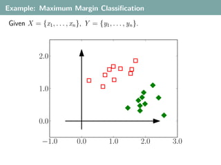
  • 13. Example: Maximum Margin Classification Given X = {x1 , . . . , xn }, Y = {y1 , . . . , yn }. 2.0 1.0 0.0 −1.0 0.0 1.0 2.0 3.0
  • 14. Example: Maximum Margin Classification Given X = {x1 , . . . , xn }, Y = {y1 , . . . , yn }. Any w partitions the data space into two half-spaces, i.e. defines a classifier. 2.0 f (x) > 0 f (x) < 0 1.0 w 0.0 −1.0 0.0 1.0 2.0 3.0 “What’s the best w?”
  • 15. Example: Maximum Margin Classification Given X = {x1 , . . . , xn }, Y = {y1 , . . . , yn }. What’s the best w? 2.0 2.0 1.0 1.0 0.0 0.0 −1.0 0.0 1.0 2.0 3.0 −1.0 0.0 1.0 2.0 3.0 Not these, since they misclassify many examples. Criterion 1: Enforce sign w, xi = yi for i = 1, . . . , n.
  • 16. Example: Maximum Margin Classification Given X = {x1 , . . . , xn }, Y = {y1 , . . . , yn }. What’s the best w? 2.0 2.0 1.0 1.0 0.0 0.0 −1.0 0.0 1.0 2.0 3.0 −1.0 0.0 1.0 2.0 3.0 Better not these, since they would be “risky” for future samples. Criterion 2: Try to ensure sign w, x = y for future (x, y) as well.
  • 17. Example: Maximum Margin Classification Given X = {x1 , . . . , xn }, Y = {y1 , . . . , yn }. Assume that future samples are similar to current ones. What’s the best w? 2.0 γ γ 1.0 0.0 −1.0 0.0 1.0 2.0 3.0 Maximize “stability”: use w such that we can maximally perturb the input samples without introducing misclassifications.
  • 18. Example: Maximum Margin Classification Given X = {x1 , . . . , xn }, Y = {y1 , . . . , yn }. Assume that future samples are similar to current ones. What’s the best w? 2.0 2.0 n rgi ma ion γ γ γ reg 1.0 1.0 0.0 0.0 −1.0 0.0 1.0 2.0 3.0 −1.0 0.0 1.0 2.0 3.0 Maximize “stability”: use w such that we can maximally perturb the input samples without introducing misclassifications. Central quantity: w margin(x) = distance of x to decision hyperplane = w ,x
  • 19. Example: Maximum Margin Classification Maximum-margin solution is determined by a maximization problem: max γ w∈Rd ,γ∈R+ subject to sign w, xi = yi for i = 1, . . . n. w , xi ≥γ for i = 1, . . . n. w Classify new samples using f (x) = w, x .
  • 20. Example: Maximum Margin Classification Maximum-margin solution is determined by a maximization problem: max γ w∈Rd , w =1 γ∈R subject to yi w, xi ≥ γ for i = 1, . . . n. Classify new samples using f (x) = w, x .
  • 21. Example: Maximum Margin Classification We can rewrite this as a minimization problem: 2 mind w w∈R subject to yi w, xi ≥ 1 for i = 1, . . . n. Classify new samples using f (x) = w, x .
  • 22. Example: Maximum Margin Classification From the view of optimization theory 2 mind w w∈R subject to yi w, xi ≥ 1 for i = 1, . . . n is rather easy: The objective function is differentiable and convex. The constraints are all linear. We can find the globally optimal w in O(n 3 ) (or faster).
  • 23. Linear Separability What is the best w for this dataset? height width
  • 24. Linear Separability What is the best w for this dataset? height width Not this.
  • 25. Linear Separability What is the best w for this dataset? height width Not this.
  • 26. Linear Separability What is the best w for this dataset? height width Not this.
  • 27. Linear Separability What is the best w for this dataset? height width Not this.
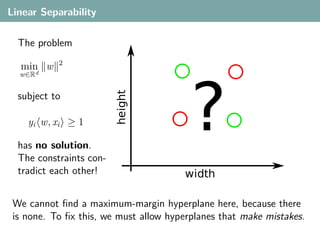
  • 28. Linear Separability The problem 2 min w ? w∈Rd height subject to yi w, xi ≥ 1 has no solution. The constraints con- tradict each other! width We cannot find a maximum-margin hyperplane here, because there is none. To fix this, we must allow hyperplanes that make mistakes.
  • 29. Linear Separability What is the best w for this dataset? height width
  • 30. Linear Separability What is the best w for this dataset? n a tio ol vi in height a rg m ξ width Possibly this one, even though one sample is misclassified.
  • 31. Linear Separability What is the best w for this dataset? height width
  • 32. Linear Separability What is the best w for this dataset? small in marg ve r y height width Maybe not this one, even though all points are classified correctly.
  • 33. Linear Separability What is the best w for this dataset? n tio height a ol vi in a rg m ξ width Trade-off: large margin vs. few mistakes on training set
  • 34. Solving for Soft-Margin Solution Mathematically, we formulate the trade-off by slack-variables ξi : n 2 min w +C ξi w∈R ,ξi ∈R+ d i=1 subject to yi w, xi ≥ 1 − ξi for i = 1, . . . n. We can fulfill every constraint by choosing ξi large enough. The larger ξi , the larger the objective (that we try to minimize). C is a regularization/trade-off parameter: small C → constraints are easily ignored large C → constraints are hard to ignore C = ∞ → hard margin case → no training error Note: The problem is still convex and efficiently solvable.
  • 35. Linear Separability So, what is the best soft-margin w for this dataset? y x None. We need something non-linear!
  • 36. Non-Linear Classification: Stacking Idea 1) Use classifier output as input to other (linear) classifiers: fi=<wi,x> σ(f5(x')) σ(f1(x)) σ(f2(x)) σ(f3(x)) σ(f4(x)) Multilayer Perceptron (Artificial Neural Network) or Boosting ⇒ decisions depend non-linearly on x and wj .
  • 37. Non-linearity: Data Preprocessing Idea 2) Preprocess the data: y This dataset is not (well) linearly separable: x θ This one is: r In fact, both are the same dataset! Top: Cartesian coordinates. Bottom: polar coordinates
  • 38. Non-linearity: Data Preprocessing y Non-linear separation x θ Linear separation r Linear classifier in polar space; acts non-linearly in Cartesian space.
  • 39. Generalized Linear Classifier Given X = {x1 , . . . , xn }, Y = {y1 , . . . , yn }. Given any (non-linear) feature map ϕ : Rk → Rm . Solve the minimization for ϕ(x1 ), . . . , ϕ(xn ) instead of x1 , . . . , xn : n 2 min w +C ξi w∈R ,ξi ∈R+ m i=1 subject to yi w, ϕ(xi ) ≥ 1 − ξi for i = 1, . . . n. The weight vector w now comes from the target space Rm . Distances/angles are measure by the scalar product . , . in Rm . Classifier f (x) = w, ϕ(x) is linear in w, but non-linear in x.
  • 40. Example Feature Mappings Polar coordinates: √ x x 2 + y2 ϕ: → y ∠(x, y) d-th degree polynomials: 2 2 d d ϕ : x1 , . . . , xn → 1, x1 , . . . , xn , x1 , . . . , xn , . . . , x1 , . . . , xn Distance map: ϕ:x→ x − pi , . . . , x − pN for a set of N prototype vectors pi , i = 1, . . . , N .
  • 41. Is this enough? In this example, changing the coordinates did help. Does this trick always work? y θ x r ↔
  • 42. Is this enough? In this example, changing the coordinates did help. Does this trick always work? y θ x r ↔ Answer: In a way, yes! Lemma Let (xi )i=1,...,n with xi = xj for i = j. Let ϕ : Rk → Rm be a feature map. If the set ϕ(xi )i=1,...,n is linearly independent, then the points ϕ(xi )i=1,...,n are linearly separable. Lemma If we choose m > n large enough, we can always find a map ϕ.
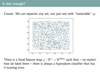
  • 43. Is this enough? Caveat: We can separate any set, not just one with “reasonable” yi : There is a fixed feature map ϕ : R2 → R20001 such that – no matter how we label them – there is always a hyperplane classifier that has zero training error.
  • 44. Is this enough? Caveat: We can separate any set, not just one with “reasonable” yi : There is a fixed feature map ϕ : R2 → R20001 such that – no matter how we label them – there is always a hyperplane classifier that has 0 training error.
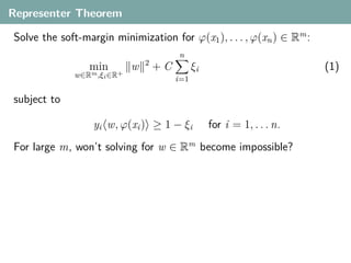
  • 45. Representer Theorem Solve the soft-margin minimization for ϕ(x1 ), . . . , ϕ(xn ) ∈ Rm : n 2 min w +C ξi (1) w∈Rm ,ξi ∈R+ i=1 subject to yi w, ϕ(xi ) ≥ 1 − ξi for i = 1, . . . n. For large m, won’t solving for w ∈ Rm become impossible?
  • 46. Representer Theorem Solve the soft-margin minimization for ϕ(x1 ), . . . , ϕ(xn ) ∈ Rm : n 2 min w +C ξi (1) w∈Rm ,ξi ∈R+ i=1 subject to yi w, ϕ(xi ) ≥ 1 − ξi for i = 1, . . . n. For large m, won’t solving for w ∈ Rm become impossible? No! Theorem (Representer Theorem) The minimizing solution w to problem (1) can always be written as n w= αj ϕ(xj ) for coefficients α1 , . . . , αn ∈ R. j=1
  • 47. Kernel Trick The representer theorem allows us to rewrite the optimization: n 2 min w +C ξi w∈R ,ξi ∈R+ m i=1 subject to yi w, ϕ(xi ) ≥ 1 − ξi for i = 1, . . . n. n Insert w = j=1 αj ϕ(xj ):
  • 48. Kernel Trick We can minimize over αi instead of w: n n 2 min αj ϕ(xj ) +C ξi αi ∈R,ξi ∈R+ j=1 i=1 subject to n yi αj ϕ(xj ), ϕ(xi ) ≥ 1 − ξi for i = 1, . . . n. j=1
  • 49. Kernel Trick 2 Use w = w, w : n n min αj αk ϕ(xj ), ϕ(xk ) + C ξi αi ∈R,ξi ∈R+ j,k=1 i=1 subject to n yi αj ϕ(xj ), ϕ(xi ) ≥ 1 − ξi for i = 1, . . . n. j=1 Note: ϕ only occurs in ϕ(.), ϕ(.) pairs.
  • 50. Kernel Trick Set ϕ(x), ϕ(x ) =: k(x, x ), called kernel function. n n min αj αk k(xj , xk ) + C ξi αi ∈R,ξi ∈R+ j,k=1 i=1 subject to n yi αj k(xj , xi ) ≥ 1 − ξi for i = 1, . . . n. j=1 The maximum-margin classifier in this form with a kernel function is often called Support-Vector Machine (SVM).
  • 51. Why use k(x, x ) instead of ϕ(x), ϕ(x ) ? 1) Speed: We might find an expression for k(xi , xj ) that is faster to calculate than forming ϕ(xi ) and then ϕ(xi ), ϕ(xj ) . Example: 2nd-order polynomial kernel (here for x ∈ R1 ): √ ϕ : x → (1, 2x, x 2 ) ∈ R3 √ √ ϕ(xi ), ϕ(xj ) = (1, 2xi , xi2 ), (1, 2xj , xj2 ) = 1 + 2xi xj + xi2 xj2 But equivalently (and faster) we can calculate without ϕ: k(xi , xj ) : = (1 + xi xj )2 = 1 + 2xi xj + xi2 xj2
  • 52. Why use k(x, x ) instead of ϕ(x), ϕ(x ) ? 2) Flexibility: There are kernel functions k(xi , xj ), for which we know that a feature transformation ϕ exists, but we don’t know what ϕ is.
  • 53. Why use k(x, x ) instead of ϕ(x), ϕ(x ) ? 2) Flexibility: There are kernel functions k(xi , xj ), for which we know that a feature transformation ϕ exists, but we don’t know what ϕ is. How that??? Theorem Let k : X × X → R be a positive definite kernel function. Then there exists a Hilbert Space H and a mapping ϕ : X → H such that k(x, x ) = ϕ(x), ϕ(x ) H where . , . H is the inner product in H.
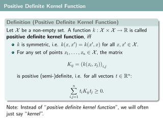
  • 54. Positive Definite Kernel Function Definition (Positive Definite Kernel Function) Let X be a non-empty set. A function k : X × X → R is called positive definite kernel function, iff k is symmetric, i.e. k(x, x ) = k(x , x) for all x, x ∈ X . For any set of points x1 , . . . , xn ∈ X , the matrix Kij = (k(xi , xj ))i,j is positive (semi-)definite, i.e. for all vectors t ∈ Rn : n ti Kij tj ≥ 0. i,j=1 Note: Instead of “positive definite kernel function”, we will often just say “kernel”.
  • 55. Hilbert Spaces Definition (Hilbert Space) A Hilbert Space H is a vector space H with an inner product . , . H , e.g. a mapping .,. H : H × H → R which is symmetric: v, v H = v , v H for all v, v ∈ H , positive definite: v, v H ≥ 0 for all v ∈ H , where v, v H = 0 only for v = 0 ∈ H . bilinear: av, v H = a v, v H for v ∈ H , a ∈ R v + v , v H = v, v H + v , v H We can treat a Hilbert space like some Rn , if we only use concepts like vectors, angles, distances. Note: dim H = ∞ is possible!
  • 56. Kernels for Arbitrary Sets Theorem Let k : X × X → R be a positive definite kernel function. Then there exists a Hilbert Space H and a mapping ϕ : X → H such that k(x, x ) = ϕ(x), ϕ(x ) H where . , . H is the inner product in H. Translation Take any set X and any function k : X × X → R. If k is a positive definite kernel, then we can use k to learn a (soft) maximum-margin classifier for the elements in X ! Note: X can be any set, e.g. X = { all images }.
  • 57. How to Check if a Function is a Kernel Problem: Checking if a given k : X × X → R fulfills the conditions for a kernel is difficult: We need to prove or disprove n ti k(xi , xj )tj ≥ 0. i,j=1 for any set x1 , . . . , xn ∈ X and any t ∈ Rn for any n ∈ N. Workaround: It is easy to construct functions k that are positive definite kernels.
  • 58. Constructing Kernels 1) We can construct kernels from scratch: For any ϕ : X → Rm , k(x, x ) = ϕ(x), ϕ(x ) Rm is a kernel. If d : X × X → R is a distance function, i.e. • d(x, x ) ≥ 0 for all x, x ∈ X , • d(x, x ) = 0 only for x = x , • d(x, x ) = d(x , x) for all x, x ∈ X , • d(x, x ) ≤ d(x, x ) + d(x , x ) for all x, x , x ∈ X , then k(x, x ) := exp(−d(x, x )) is a kernel.
  • 59. Constructing Kernels 1) We can construct kernels from scratch: For any ϕ : X → Rm , k(x, x ) = ϕ(x), ϕ(x ) Rm is a kernel. If d : X × X → R is a distance function, i.e. • d(x, x ) ≥ 0 for all x, x ∈ X , • d(x, x ) = 0 only for x = x , • d(x, x ) = d(x , x) for all x, x ∈ X , • d(x, x ) ≤ d(x, x ) + d(x , x ) for all x, x , x ∈ X , then k(x, x ) := exp(−d(x, x )) is a kernel. 2) We can construct kernels from other kernels: if k is a kernel and α > 0, then αk and k + α are kernels. if k1 , k2 are kernels, then k1 + k2 and k1 · k2 are kernels.
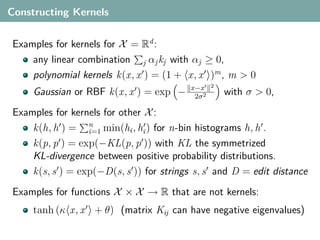
  • 60. Constructing Kernels Examples for kernels for X = Rd : any linear combination j αj kj with αj ≥ 0, polynomial kernels k(x, x ) = (1 + x, x )m , m > 0 x−x 2 Gaussian or RBF k(x, x ) = exp − 2σ 2 with σ > 0,
  • 61. Constructing Kernels Examples for kernels for X = Rd : any linear combination j αj kj with αj ≥ 0, polynomial kernels k(x, x ) = (1 + x, x )m , m > 0 x−x 2 Gaussian or RBF k(x, x ) = exp − 2σ 2 with σ > 0, Examples for kernels for other X : k(h, h ) = n min(hi , hi ) for n-bin histograms h, h . i=1 k(p, p ) = exp(−KL(p, p )) with KL the symmetrized KL-divergence between positive probability distributions. k(s, s ) = exp(−D(s, s )) for strings s, s and D = edit distance
  • 62. Constructing Kernels Examples for kernels for X = Rd : any linear combination j αj kj with αj ≥ 0, polynomial kernels k(x, x ) = (1 + x, x )m , m > 0 x−x 2 Gaussian or RBF k(x, x ) = exp − 2σ 2 with σ > 0, Examples for kernels for other X : k(h, h ) = n min(hi , hi ) for n-bin histograms h, h . i=1 k(p, p ) = exp(−KL(p, p )) with KL the symmetrized KL-divergence between positive probability distributions. k(s, s ) = exp(−D(s, s )) for strings s, s and D = edit distance Examples for functions X × X → R that are not kernels: tanh (κ x, x + θ) (matrix Kij can have negative eigenvalues)
  • 63. Kernels in Computer Vision X = { images }, treat feature extraction as part of kernel definition OCR/handwriting recognition resize image, normalize brightness/contrast/rotation/skew polynomial kernel k(x, x ) = (1 + x, x )d , d > 0 [DeCoste, Schölkopf. ML2002] Pedestrian detection resize image, calculate local intensity gradient directions local thresholding + linear kernel [Dalal, Triggs. CVPR 2005] or local L1 -normalization + histogram intersection kernel [Maji, Berg, Malik. CVPR 2008]
  • 64. Kernels in Computer Vision X = { images }, treat feature extraction as part of kernel definition object category recognition extract local image descriptors, e.g. SIFT calculate multi-level pyramid histograms h l,k (x) pyramid match kernel [Grauman, Darrell. ICCV 2005] L 2l−1 l kPMK (x, x ) = 2 min h l,k (x), h l,k (x ) l=1 k=1 scene/object category recognition extract local image descriptors, e.g. SIFT quantize descriptors into bag-of-words histograms χ2 -kernel [Puzicha, Buhmann, Rubner, Tomasi. ICCV1999] kχ2 (h, h ) = exp −γχ2 (h, h ) for γ > 0 K (hk − hk )2 χ2 (h, h ) = k=1 hk + hk
  • 65. Summary Linear methods are popular and well understood classification, regression, dimensionality reduction, ... Kernels are at the same time... 1) Similarity measure between (arbitrary) objects, 2) Scalar products in a (hidden) vector space. Kernelization can make linear techniques more powerful implicit preprocessing, non-linear in the original data. still linear in some feature space ⇒ still intuitive/interpretable Kernels can be defined over arbitrary inputs, e.g. images unified framework for all preprocessing steps different features, normalization, etc., becomes kernel choices
  • 66. What did we not see? We have skipped the largest part of theory on kernel methods: Optimization Dualization Algorithms to train SVMs Kernel Design Systematic methods to construct data-dependent kernels. Statistical Interpretations What do we assume about samples? What performance can we expect? Generalization Bounds The test error of a (kernelized) linear classifier can be controlled using its modelling error and its training error. “Support Vectors” This and much more in standard references.
  • 68. Selecting From Multiple Kernels Typically, one has many different kernels to choose from: different functional forms linear, polynomial, RBF, . . . different parameters polynomial degree, Gaussian bandwidth, . . .
  • 69. Selecting From Multiple Kernels Typically, one has many different kernels to choose from: different functional forms linear, polynomial, RBF, . . . different parameters polynomial degree, Gaussian bandwidth, . . . Different image features give rise to different kernels Color histograms, SIFT bag-of-words, HOG, Pyramid match, Spatial pyramids, . . .
  • 70. Selecting From Multiple Kernels Typically, one has many different kernels to choose from: different functional forms linear, polynomial, RBF, . . . different parameters polynomial degree, Gaussian bandwidth, . . . Different image features give rise to different kernels Color histograms, SIFT bag-of-words, HOG, Pyramid match, Spatial pyramids, . . . How to choose? Ideally, based on the kernels’ performance on task at hand: estimate by cross-validation or validation set error Classically part of “Model Selection”.
  • 71. Kernel Parameter Selection Note: Model Selection makes a difference! Action Classification, KTH dataset Method Accuracy Dollár et al. VS-PETS 2005: ”SVM classifier“ 80.66 Nowozin et al., ICCV 2007: ”baseline RBF“ 85.19 identical features, same kernel function difference: Nowozin used cross-validation for model selection (bandwidth and C ) Note: there is no overfitting involved here. Model selection is fully automatic and uses only training data.
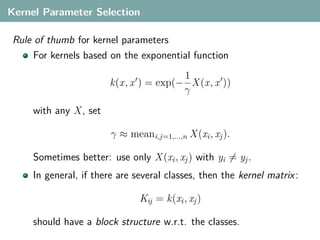
  • 72. Kernel Parameter Selection Rule of thumb for kernel parameters For kernels based on the exponential function 1 k(x, x ) = exp(− X (x, x )) γ with any X , set γ ≈ meani,j=1,...,n X (xi , xj ). Sometimes better: use only X (xi , xj ) with yi = yj . In general, if there are several classes, then the kernel matrix : Kij = k(xi , xj ) should have a block structure w.r.t. the classes.
  • 73. 1.0 1.0 0 0.9 0 0 0.9 2.4 1.0 y 0.8 0.8 10 10 1.6 10 0.7 0.7 0.5 x 20 0.6 20 0.8 20 0.6 0.5 0.5 0.0 0.0 30 0.4 30 30 0.4 −0.8 −0.5 0.3 0.3 40 0.2 40 −1.6 40 0.2 −1.0 0.1 −2.4 0.1 −2.0 −1.0 0.0 1.0 2.0 0 10 20 30 40 50 0.0 0 10 20 30 40 50 0 10 20 30 40 50 0.0 two moons label “kernel” linear RBF: γ = 0.001 1.0 1.0 1.0 1.0 0 0.9 0 0.9 0 0.9 0 0.9 0.8 0.8 0.8 0.8 10 10 10 10 0.7 0.7 0.7 0.7 20 0.6 20 0.6 20 0.6 20 0.6 0.5 0.5 0.5 0.5 30 0.4 30 0.4 30 0.4 30 0.4 0.3 0.3 0.3 0.3 40 0.2 40 0.2 40 0.2 40 0.2 0.1 0.1 0.1 0.1 0 10 20 30 40 50 0.0 0 10 20 30 40 50 0.0 0 10 20 30 40 50 0.0 0 10 20 30 40 50 0.0 γ = 0.01 γ = 0.1 γ=1 γ = 10 1.0 1.0 0 0.9 0 0.9 0.8 0.8 10 10 0.7 0.7 20 0.6 20 0.6 0.5 0.5 30 0.4 30 0.4 0.3 0.3 40 0.2 40 0.2 0.1 0.1 0 10 20 30 40 50 0.0 0 10 20 30 40 50 0.0 γ = 100 γ = 1000
  • 74. 1.0 1.0 0 0.9 0 0 0.9 2.4 1.0 y 0.8 0.8 10 10 1.6 10 0.7 0.7 0.5 x 20 0.6 20 0.8 20 0.6 0.5 0.5 0.0 0.0 30 0.4 30 30 0.4 −0.8 −0.5 0.3 0.3 40 0.2 40 −1.6 40 0.2 −1.0 0.1 −2.4 0.1 −2.0 −1.0 0.0 1.0 2.0 0 10 20 30 40 50 0.0 0 10 20 30 40 50 0 10 20 30 40 50 0.0 two moons label “kernel” linear RBF: γ = 0.001 1.0 1.0 1.0 1.0 0 0.9 0 0.9 0 0.9 0 0.9 0.8 0.8 0.8 0.8 10 10 10 10 0.7 0.7 0.7 0.7 20 0.6 20 0.6 20 0.6 20 0.6 0.5 0.5 0.5 0.5 30 0.4 30 0.4 30 0.4 30 0.4 0.3 0.3 0.3 0.3 40 0.2 40 0.2 40 0.2 40 0.2 0.1 0.1 0.1 0.1 0 10 20 30 40 50 0.0 0 10 20 30 40 50 0.0 0 10 20 30 40 50 0.0 0 10 20 30 40 50 0.0 γ = 0.01 γ = 0.1 γ=1 γ = 10 1.0 1.0 1.0 0 0.9 0 0.9 0 0.9 0.8 0.8 0.8 10 10 10 0.7 0.7 0.7 20 0.6 20 0.6 20 0.6 0.5 0.5 0.5 30 0.4 30 0.4 30 0.4 0.3 0.3 0.3 40 0.2 40 0.2 40 0.2 0.1 0.1 0.1 0 10 20 30 40 50 0.0 0 10 20 30 40 50 0.0 0 10 20 30 40 50 0.0 γ = 100 γ = 1000 γ = 0.6 rule of thumb
  • 75. 1.0 1.0 0 0.9 0 0 0.9 2.4 1.0 y 0.8 0.8 10 10 1.6 10 0.7 0.7 0.5 x 20 0.6 20 0.8 20 0.6 0.5 0.5 0.0 0.0 30 0.4 30 30 0.4 −0.8 −0.5 0.3 0.3 40 0.2 40 −1.6 40 0.2 −1.0 0.1 −2.4 0.1 −2.0 −1.0 0.0 1.0 2.0 0 10 20 30 40 50 0.0 0 10 20 30 40 50 0 10 20 30 40 50 0.0 two moons label “kernel” linear RBF: γ = 0.001 1.0 1.0 1.0 1.0 0 0.9 0 0.9 0 0.9 0 0.9 0.8 0.8 0.8 0.8 10 10 10 10 0.7 0.7 0.7 0.7 20 0.6 20 0.6 20 0.6 20 0.6 0.5 0.5 0.5 0.5 30 0.4 30 0.4 30 0.4 30 0.4 0.3 0.3 0.3 0.3 40 0.2 40 0.2 40 0.2 40 0.2 0.1 0.1 0.1 0.1 0 10 20 30 40 50 0.0 0 10 20 30 40 50 0.0 0 10 20 30 40 50 0.0 0 10 20 30 40 50 0.0 γ = 0.01 γ = 0.1 γ=1 γ = 10 1.0 1.0 1.0 1.0 0 0.9 0 0.9 0 0.9 0 0.9 0.8 0.8 0.8 0.8 10 10 10 10 0.7 0.7 0.7 0.7 20 0.6 20 0.6 20 0.6 20 0.6 0.5 0.5 0.5 0.5 30 0.4 30 0.4 30 0.4 30 0.4 0.3 0.3 0.3 0.3 40 0.2 40 0.2 40 0.2 40 0.2 0.1 0.1 0.1 0.1 0 10 20 30 40 50 0.0 0 10 20 30 40 50 0.0 0 10 20 30 40 50 0.0 0 10 20 30 40 50 0.0 γ = 100 γ = 1000 γ = 0.6 γ = 1.6 rule of thumb 5-fold CV
  • 76. Kernel Selection ↔ Kernel Combination Is there a single best kernel at all? Kernels are typcally designed to capture one aspect of the data texture, color, edges, . . . Choosing one kernel means to select exactly one such aspect.
  • 77. Kernel Selection ↔ Kernel Combination Is there a single best kernel at all? Kernels are typcally designed to capture one aspect of the data texture, color, edges, . . . Choosing one kernel means to select exactly one such aspect. Combining aspects if often better than Selecting. Method Accuracy Colour 60.9 ± 2.1 Shape 70.2 ± 1.3 Texture 63.7 ± 2.7 HOG 58.5 ± 4.5 HSV 61.3 ± 0.7 siftint 70.6 ± 1.6 siftbdy 59.4 ± 3.3 combination 85.2 ± 1.5 Mean accuracy on Oxford Flowers dataset [Gehler, Nowozin: ICCV2009]
  • 78. Combining Two Kernels For two kernels k1 , k2 : product k = k1 k2 is again a kernel Problem: very small kernel values suppress large ones average k = 1 (k1 + k2 ) is again a kernel 2 Problem: k1 , k2 on different scales. Re-scale first? convex combination kβ = (1 − β)k1 + βk2 with β ∈ [0, 1] Model selection: cross-validate over β ∈ {0, 0.1, . . . , 1}.
  • 79. Combining Many Kernels Multiple kernels: k1 ,. . . ,kK all convex combinations are kernels: K K k= βj kj with βj ≥ 0, β = 1. j=1 j=1 Kernels can be “deactivated” by βj = 0. Combinatorial explosion forbids cross-validation over all combinations of βj Proxy: instead of CV, maximize SVM-objective. Each combined kernel induces a feature space. In which of the feature spaces can we best explain the training data, and achieve a large margin between the classes?
  • 80. Feature Space View of Kernel Combination Each kernel kj induces a Hilbert Space Hj and a mapping ϕj : X → Hj . β The weighted kernel kj j := βj kj induces the same Hilbert Space Hj , but β a rescaled feature mapping ϕj j (x) := βj ϕj (x). β β k βj (x, x ) ≡ ϕj j (x), ϕj j (x ) H = βj ϕj (x), βj ϕj (x ) H = βj ϕj (x), ϕj (x ) H = βj k(x, x ). ˆ The linear combination k := K βj kj induces j=1 the product space H := ⊕K Hj , and j=1 the product mapping ϕ(x) := (ϕβ1 (x), . . . , ϕβn (x))t ˆ 1 n K K ˆ β β k(x, x ) ≡ ϕ(x), ϕ(x ) ˆ ˆ H = ϕj j (x), ϕj j (x ) H = βj k(x, x ) j=1 j=1
  • 81. Feature Space View of Kernel Combination Implicit representation of a dataset using two kernels: Kernel k1 , feature representation ϕ1 (x1 ), . . . , ϕ1 (xn ) ∈ H1 Kernel k2 , feature representation ϕ2 (x1 ), . . . , ϕ2 (xn ) ∈ H2 Kernel Selection would most likely pick k2 . For k = (1 − β)k1 + βk2 , top is β = 0, bottom is β = 1.
  • 82. Feature Space View of Kernel Combination β = 0.00 margin = 0.0000 5 √ 1.00φ2 (xi ) H1 × H2 4 3 2 1 0 √ 0.00φ1 (xi ) −1 −1 0 1 2 3 4 5
  • 83. Feature Space View of Kernel Combination β = 1.00 margin = 0.1000 5 √ 0.00φ2 (xi ) H1 × H2 4 3 2 1 0 √ 1.00φ1 (xi ) −1 −1 0 1 2 3 4 5
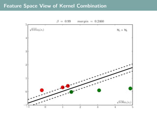
  • 84. Feature Space View of Kernel Combination β = 0.99 margin = 0.2460 5 √ 0.01φ2 (xi ) H1 × H2 4 3 2 1 0 √ 0.99φ1 (xi ) −1 −1 0 1 2 3 4 5
  • 85. Feature Space View of Kernel Combination β = 0.98 margin = 0.3278 5 √ 0.02φ2 (xi ) H1 × H2 4 3 2 1 0 √ 0.98φ1 (xi ) −1 −1 0 1 2 3 4 5
  • 86. Feature Space View of Kernel Combination β = 0.97 margin = 0.3809 5 √ 0.03φ2 (xi ) H1 × H2 4 3 2 1 0 √ 0.97φ1 (xi ) −1 −1 0 1 2 3 4 5
  • 87. Feature Space View of Kernel Combination β = 0.95 margin = 0.4515 5 √ 0.05φ2 (xi ) H1 × H2 4 3 2 1 0 √ 0.95φ1 (xi ) −1 −1 0 1 2 3 4 5
  • 88. Feature Space View of Kernel Combination β = 0.90 margin = 0.5839 5 √ 0.10φ2 (xi ) H1 × H2 4 3 2 1 0 √ 0.90φ1 (xi ) −1 −1 0 1 2 3 4 5
  • 89. Feature Space View of Kernel Combination β = 0.80 margin = 0.7194 5 √ 0.20φ2 (xi ) H1 × H2 4 3 2 1 0 √ 0.80φ1 (xi ) −1 −1 0 1 2 3 4 5
  • 90. Feature Space View of Kernel Combination β = 0.70 margin = 0.7699 5 √ 0.30φ2 (xi ) H1 × H2 4 3 2 1 0 √ 0.70φ1 (xi ) −1 −1 0 1 2 3 4 5
  • 91. Feature Space View of Kernel Combination β = 0.65 margin = 0.7770 5 √ 0.35φ2 (xi ) H1 × H2 4 3 2 1 0 √ 0.65φ1 (xi ) −1 −1 0 1 2 3 4 5
  • 92. Feature Space View of Kernel Combination β = 0.60 margin = 0.7751 5 √ 0.40φ2 (xi ) H1 × H2 4 3 2 1 0 √ 0.60φ1 (xi ) −1 −1 0 1 2 3 4 5
  • 93. Feature Space View of Kernel Combination β = 0.50 margin = 0.7566 5 √ 0.50φ2 (xi ) H1 × H2 4 3 2 1 0 √ 0.50φ1 (xi ) −1 −1 0 1 2 3 4 5
  • 94. Feature Space View of Kernel Combination β = 0.40 margin = 0.7365 5 √ 0.60φ2 (xi ) H1 × H2 4 3 2 1 0 √ 0.40φ1 (xi ) −1 −1 0 1 2 3 4 5
  • 95. Feature Space View of Kernel Combination β = 0.30 margin = 0.7073 5 √ 0.70φ2 (xi ) H1 × H2 4 3 2 1 0 √ 0.30φ1 (xi ) −1 −1 0 1 2 3 4 5
  • 96. Feature Space View of Kernel Combination β = 0.20 margin = 0.6363 5 √ 0.80φ2 (xi ) H1 × H2 4 3 2 1 0 √ 0.20φ1 (xi ) −1 −1 0 1 2 3 4 5
  • 97. Feature Space View of Kernel Combination β = 0.10 margin = 0.4928 5 √ 0.90φ2 (xi ) H1 × H2 4 3 2 1 0 √ 0.10φ1 (xi ) −1 −1 0 1 2 3 4 5
  • 98. Feature Space View of Kernel Combination β = 0.03 margin = 0.2870 5 √ 0.97φ2 (xi ) H1 × H2 4 3 2 1 0 √ 0.03φ1 (xi ) −1 −1 0 1 2 3 4 5
  • 99. Feature Space View of Kernel Combination β = 0.02 margin = 0.2363 5 √ 0.98φ2 (xi ) H1 × H2 4 3 2 1 0 √ 0.02φ1 (xi ) −1 −1 0 1 2 3 4 5
  • 100. Feature Space View of Kernel Combination β = 0.01 margin = 0.1686 5 √ 0.99φ2 (xi ) H1 × H2 4 3 2 1 0 √ 0.01φ1 (xi ) −1 −1 0 1 2 3 4 5
  • 101. Feature Space View of Kernel Combination β = 0.00 margin = 0.0000 5 √ 1.00φ2 (xi ) H1 × H2 4 3 2 1 0 √ 0.00φ1 (xi ) −1 −1 0 1 2 3 4 5
  • 102. Multiple Kernel Learning Can we calculate coefficients βj that realize the largest margin? Analyze: how does the margin depend on βj ? Remember standard SVM (here without slack variables): 2 min w H w∈H subject to yi w, xi H ≥1 for i = 1, . . . n. H and ϕ were induced by kernel k. New samples are classified by f (x) = w, x H.
  • 103. Multiple Kernel Learning Insert K k(x, x ) = βj kj (x, x ) (2) j=1 with Hilbert space H = ⊕j√ j , H √ feature map ϕ(x) = ( β1 ϕ1 (x), . . . , βK ϕK (x))t , weight vector w = (w1 , . . . , wK )t . such that 2 2 w H = wj Hj (3) j w, ϕ(xi ) H = βj wj , ϕj (xi ) Hj (4) j
  • 104. Multiple Kernel Learning For fixed βj , the largest margin hyperplane is given by 2 min wj Hj wj ∈Hj j subject to yi βj wj , ϕj (xi ) Hj ≥1 for i = 1, . . . n. j 0 Renaming vj = βj wj (and defining 0 = 0): 1 2 min vj Hj vj ∈Hj j βj subject to yi vj , ϕj (xi ) Hj ≥1 for i = 1, . . . n. j
  • 105. Multiple Kernel Learning Therefore, best hyperplane for variable βj is given by: 1 2 min vj Hj (5) vj ∈Hj j βj β =1 j j βj ≥0 subject to yi vj , ϕj (xi ) Hj ≥1 for i = 1, . . . n. (6) j This optimization problem is jointly-convex in vj and βj . There is a unique global minimum, and we can find it efficiently!
  • 106. Multiple Kernel Learning Same for soft-margin with slack-variables: 1 2 min vj Hj +C ξi (7) vj ∈Hj j βj i β =1 j j βj ≥0 ξi ∈R+ subject to yi vj , ϕj (xi ) Hj ≥ 1 − ξi for i = 1, . . . n. (8) j This optimization problem is jointly-convex in vj and βj . There is a unique global minimum, and we can find it efficiently!
  • 107. Software for Multiple Kernel Learning Existing toolboxes allow Multiple-Kernel SVM training: Shogun (C++ with bindings to Matlab, Python etc.) http://www.fml.tuebingen.mpg.de/raetsch/projects/shogun MPI IKL (Matlab with libSVM, CoinIPopt) http://www.kyb.mpg.de/bs/people/pgehler/ikl-webpage/index.html SimpleMKL (Matlab) http://asi.insa-rouen.fr/enseignants/˜arakotom/code/mklindex.html SKMsmo (Matlab) http://www.di.ens.fr/˜fbach/ (older and slower than the others) Typically, one only has to specify the set of candidate kernels and the regularization parameter C .
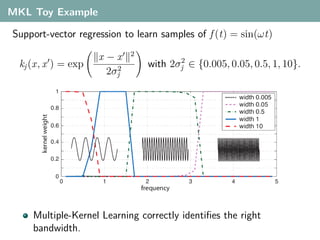
  • 108. MKL Toy Example Support-vector regression to learn samples of f (t) = sin(ωt) 2 x −x 2 kj (x, x ) = exp 2 with 2σj ∈ {0.005, 0.05, 0.5, 1, 10}. 2σj Multiple-Kernel Learning correctly identifies the right bandwidth.
  • 109. Combining Good Kernels Observation: if all kernels are reasonable, simple combination methods work as well as difficult ones (and are much faster): Single features Combination methods Method Accuracy Time Method Accuracy Time Colour 60.9 ± 2.1 3 product 85.5 ± 1.2 2 Shape 70.2 ± 1.3 4 averaging 84.9 ± 1.9 10 Texture 63.7 ± 2.7 3 CG-Boost 84.8 ± 2.2 1225 HOG 58.5 ± 4.5 4 MKL (SILP) 85.2 ± 1.5 97 HSV 61.3 ± 0.7 3 MKL (Simple) 85.2 ± 1.5 152 siftint 70.6 ± 1.6 4 LP-β 85.5 ± 3.0 80 siftbdy 59.4 ± 3.3 5 LP-B 85.4 ± 2.4 98 Mean accuracy and total runtime (model selection, training, testing) on Oxford Flowers dataset [Gehler, Nowozin: ICCV2009]
  • 110. Combining Good and Bad kernels Observation: if some kernels are helpful, but others are not, smart techniques are better. Performance with added noise features 90 85 80 75 accuracy 70 65 product 60 average CG−Boost 55 MKL (silp or simple) 50 LP−β LP−B 45 01 5 10 25 50 no. noise features added Mean accuracy on Oxford Flowers dataset [Gehler, Nowozin: ICCV2009]
  • 111. Example: Multi-Class Object Localization MKL for joint prediction of different object classes. Objects in images do not occur independently of each other. Chairs and tables often occur together in indoor scenes. Busses often occur together with cars in street scenes. Chairs rarely occur together with cars. One can make use of these dependencies to improve prediction.
  • 112. Example: Multi-Class Object Localization Predict candidate regions for all object classes. Train a decision function for each class (red), taking into account candidate regions for all classes (red and green). Decide per-class which other object categories are worth using 20 2 2 k(I , I ) = β0 kχ (h, h ) + βj kχ (hj , hj ) j=1 h: feature histogram for the full image x hj : histogram for the region predicted for object class j in x Use MKL to learn weights βj , j = 0, . . . , 20. [Lampert and Blaschko, DAGM 2008]
  • 113. Example: Multi-Class Object Localization Benchmark on PASCAL VOC 2006 and VOC 2007. Combination improves detection accuracy (black vs. blue).
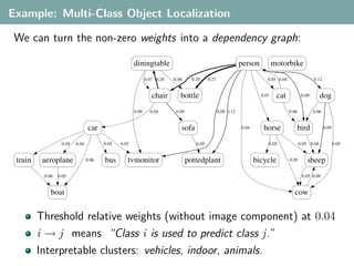
  • 114. Example: Multi-Class Object Localization Interpretation of Weights (VOC 2007): Every class decision 0 1 2 3 4 5 6 7 8 9 10 11 12 13 14 15 16 17 18 19 20 depends on the full image aeroplane [1] bicycle [2] and on the object box. bird [3] boat [4] bottle [5] bus [6] High image weights: car [7] cat [8] → scene classification? chair [9] cow [10] diningtable [11] dog [12] Intuitive connections: horse [13] motorbike [14] chair → diningtable, person [15] pottedplant [16] sheep [17] person → bottle, sofa [18] train [19] person → dog. tvmonitor [20] Many classes depend on rows: class to be detected the person class. columns: class candidate boxes
  • 115. Example: Multi-Class Object Localization We can turn the non-zero weights into a dependency graph: diningtable person motorbike 0.07 0.20 0.06 0.20 0.27 0.05 0.04 0.12 chair bottle 0.07 cat 0.09 dog 0.08 0.04 0.09 0.09 0.12 0.06 0.06 car sofa 0.04 horse bird 0.09 0.05 0.04 0.05 0.05 0.05 0.05 0.05 0.08 0.05 train aeroplane 0.06 bus tvmonitor pottedplant bicycle 0.05 sheep 0.06 0.05 0.05 0.08 boat cow Threshold relative weights (without image component) at 0.04 i → j means “Class i is used to predict class j.” Interpretable clusters: vehicles, indoor, animals.
  • 116. Summary Kernel Selection and Combination Model selection is important to achive highest accuracy Combining several kernels is often superior to selecting one Multiple-Kernel Learning Learn weights for the “best” linear kernel combination: unified approach to feature selection/combination. visit [Gehler, Nowozin. CVPR 2009] on Wednesday afternoon Beware: MKL is no silver bullet. Other and even simpler techniques might be superior! Always compare against single best, averaging, product. Warning: Caltech101/256 Be careful when reading kernel combination results Many results reported rely on “broken” Bosch kernel matrices