SlideShare a Scribd company logo
Statistics and Clustering with Kernels

      Christoph Lampert & Matthew Blaschko

         Max-Planck-Institute for Biological Cybernetics
          Department Schölkopf: Empirical Inference
                     TĂŒbingen, Germany

                    Visual Geometry Group
                     University of Oxford
                       United Kingdom


                      June 20, 2009
Overview


  Kernel Ridge Regression
  Kernel PCA
  Spectral Clustering
  Kernel Covariance and Canonical Correlation Analysis
  Kernel Measures of Independence
Kernel Ridge Regression

   Regularized least squares regression:
                         n
                   min         (yi − w, xi )2 + λ w   2
                     w
                         i=1
Kernel Ridge Regression

   Regularized least squares regression:
                                  n
                       min                (yi − w, xi )2 + λ w        2
                          w
                              i=1


                          n
   Replace w with         i=1     α i xi
                      ïŁ«                         ïŁ¶2
                n                     n                     n   n
          min         ïŁ­yi     −            xi , xj ïŁž + λ             αi αj xi , xj
            α
                i=1               j=1                      i=1 j=1


   α∗ can be solved in closed form solution

                                   α∗ = (K + λI )−1 y
PCA
Equivalent formulations:
     Minimize squared error between original data and a projection of
     our data into a lower dimensional subspace
     Maximize variance of projected data
Solutions: Eigenvectors of the empirical covariance matrix
PCA continued

  Empirical covariance matrix (biased):

                    ˆ   1
                    C =         (xi − ”)(xi − ”)T
                        n   i

  where ” is the sample mean.

  ˆ
  C is positive (semi-)deïŹnite symmetric

  PCA:
                                     ˆ
                                  wT C w
                            max
                             w     w 2
Data Centering

   We use the notation X to denote the design matrix where every
   column of X is a data sample
   We can deïŹne a centering matrix
                                     1 T
                            H =I−      ee
                                     n
   where e is a vector of all ones
Data Centering

   We use the notation X to denote the design matrix where every
   column of X is a data sample
   We can deïŹne a centering matrix
                                    1 T
                          H =I−       ee
                                    n
   where e is a vector of all ones
   H is idempotent, symmetric, and positive semi-deïŹnite (rank
   n − 1)
   The design matrix of centered data can be written compactly in
   matrix form as XH
                                                            1
       The ith column of XH is equal to xi − ”, where ” =   n   j xj   is
       the sample mean
Kernel PCA
  PCA:
                                   ˆ
                                wT C w
                            max
                             w   w 2
  Kernel PCA:
      Replace w by i αi (xi − ”) - this can be represented compactly
      in matrix form by w = XH α where X is the design matrix, H is
      the centering matrix, and α is the coeïŹƒcient vector.
                 ˆ                   ˆ    1
      Compute C in matrix form as C = n XHX T
      Denote the matrix of pairwise inner products K = X T X , i.e.
      Kij = xi , xj
                         ˆ
                     wT C w          1 αT HKHKH α
                max          = max
                 w     w 2       α n αT HKH α

  This is a Rayleigh quotient with known solution

                          HKH ÎČi = λi ÎČi
Kernel PCA
    Set ÎČ to be the eigenvectors of HKH , and λ the corresponding
    eigenvalues
                 1
    Set α = ÎČλ− 2
Example, image super-resolution:


                   (ïŹg: Kim et al., PAMI 2005.)
Overview


  Kernel Ridge Regression
  Kernel PCA
  Spectral Clustering
  Kernel Covariance and Canonical Correlation Analysis
  Kernel Measures of Independence
Spectral Clustering

   Represent similarity of images by weights on a graph
   Normalized cuts optimizes the ratio of the cost of a cut and the
   volume of each cluster
                                             k           ÂŻ
                                                cut(Ai , Ai )
                 Ncut(A1 , . . . , Ak ) =
                                            i=1   vol(Ai )
Spectral Clustering

   Represent similarity of images by weights on a graph
   Normalized cuts optimizes the ratio of the cost of a cut and the
   volume of each cluster
                                                k        ÂŻ
                                                cut(Ai , Ai )
                 Ncut(A1 , . . . , Ak ) =
                                            i=1   vol(Ai )

   Exact optimization is NP-hard, but relaxed version can be solved
   by ïŹnding the eigenvalues of the graph Laplacian
                                            1       1
                          L = I − D − 2 AD − 2

   where D is the diagonal matrix with entries equal to the row
   sums of similarity matrix, A.
Spectral Clustering (continued)
                        1     1
   Compute L = I − D − 2 AD − 2 .
   Map data points based on the eigenvalues of L
   Example, handwritten digits (0-9):


                          (ïŹg: Xiaofei He)
   Cluster in mapped space using k-means
Overview


  Kernel Ridge Regression
  Kernel PCA
  Spectral Clustering
  Kernel Covariance and Canonical Correlation Analysis
  Kernel Measures of Independence
Multimodal Data


  A latent aspect relates data that are present in multiple
  modalities
  e.g. images and text

                  XYZ[
                  _^]
                    z M
                qqq    MMM
             qqq          MMM
    XYZ[
    _^]                     _^]
                             XYZ[
           q
           x                 &
    ϕx (x)                     ϕy (y)   x:
                                        y:   “A view from Idyllwild, California,
                                        with pine trees and snow capped Marion
                                        Mountain under a blue sky.”

  Learn kernelized projections that relate both spaces
Kernel Covariance
   KPCA is maximization of auto-covariance
   Instead maximize cross-covariance
                                   wx Cxy wy
                          max
                          w ,w
                           x   y   wx wy
Kernel Covariance
   KPCA is maximization of auto-covariance
   Instead maximize cross-covariance
                                     wx Cxy wy
                            max
                            w ,w
                             x   y   wx wy

   Can also be kernelized (replace wx by         i   αi (xi − ”x ), etc.)

                                 αT HKx HKy H ÎČ
                   maxα,ÎČ
                            αT HKx H αÎČ T HKy H ÎČ

   Solution is given by (generalized) eigenproblem

         0     HKx HKy H             α    HKx H  0                          α
                                       =λ
     HKy HKx H     0                 ÎČ     0    HKy H                       ÎČ
Kernel Canonical Correlation Analysis
(KCCA)

   Alternately, maximize correlation instead of covariance
                                   T
                                  wx Cxy wy
                      max
                      wx ,wy    T         T
                               wx Cxx wx wy Cyy wy
Kernel Canonical Correlation Analysis
(KCCA)

   Alternately, maximize correlation instead of covariance
                                     T
                                    wx Cxy wy
                        max
                        wx ,wy    T         T
                                 wx Cxx wx wy Cyy wy


   Kernelization is straightforward as before

                                 αT HKx HKy H ÎČ
                 max
                  α,ÎČ
                          αT (HKx H )2 αÎČ T (HKy H )2 ÎČ
KCCA (continued)

  Problem:
  If the data in either modality are linearly independent (as many
  dimensions as data points), there exists a projection of the data
  that respects any arbitrary ordering
  Perfect correlation can always be achieved
KCCA (continued)

  Problem:
  If the data in either modality are linearly independent (as many
  dimensions as data points), there exists a projection of the data
  that respects any arbitrary ordering
  Perfect correlation can always be achieved
  This is even more likely when a kernel is used (e.g. Gaussian)

  Solution: Regularize
                                 T
                                wx Cxy wy
       max
       wx ,wy
                (wx Cxx wx + Δx wx 2 ) wy Cyy wy + Δy wy
                  T                     T                  2


  As Δx → ∞, Δx → ∞, solution approaches maximum covariance
KCCA Algorithm


  Compute Kx , Ky
  Solve for α and ÎČ as the eigenvectors of

          0     HKx HKy H         α
                                    =
      HKy HKx H     0             ÎČ
           (HKx H )2 + Δx HKx H           0           α
         λ                              2
                     0          (HKy H ) + Δy HKy H   ÎČ
Content Based Image Retrieval with KCCA


   Hardoon et al., 2004
   Training data consists of images with text captions
   Learn embeddings of both spaces using KCCA and appropriately
   chosen image and text kernels
   Retrieval consists of ïŹnding images whose embeddings are
   related to the embedding of the text query

   A kind of multi-variate regression
Overview


  Kernel Ridge Regression
  Kernel PCA
  Spectral Clustering
  Kernel Covariance and Canonical Correlation Analysis
  Kernel Measures of Independence
Kernel Measures of Independence


   We know how to measure correlation in the kernelized space
Kernel Measures of Independence


   We know how to measure correlation in the kernelized space

   Independence implies zero correlation
Kernel Measures of Independence


   We know how to measure correlation in the kernelized space

   Independence implies zero correlation

   DiïŹ€erent kernels encode diïŹ€erent statistical properties of the
   data
Kernel Measures of Independence


   We know how to measure correlation in the kernelized space

   Independence implies zero correlation

   DiïŹ€erent kernels encode diïŹ€erent statistical properties of the
   data

   Use an appropriate kernel such that zero correlation in the
   Hilbert space implies independence
Example: Polynomial Kernel
   First degree polynomial kernel (i.e. linear) captures correlation
   only
   Second degree polynomial kernel captures all second order
   statistics
   ...
Example: Polynomial Kernel
   First degree polynomial kernel (i.e. linear) captures correlation
   only
   Second degree polynomial kernel captures all second order
   statistics
   ...
   A Gaussian kernel can be written
                                         2
           k(xi , xj ) = e −γ   xi −xj
                                             = e −γ   xi ,xi
                                                               e 2Îł   xi ,xj
                                                                               e −γ   xj ,xj


   and we can use the identity
                                              ∞
                                                  1 i
                                    ez =             z
                                              i=1 i!


   We can view the Gaussian kernel as being related to an
   appropriately scaled inïŹnite dimensional polynomial kernel
        captures all order statistics
Hilbert-Schmidt Independence Criterion
   F RKHS on X with kernel kx (x, x ), G RKHS on Y with kernel
   ky (y, y )
Hilbert-Schmidt Independence Criterion
   F RKHS on X with kernel kx (x, x ), G RKHS on Y with kernel
   ky (y, y )
   Covariance operator: Cxy : G → F such that

           f , Cxy g   F   = Ex,y [f (x)g(y)] − Ex [f (x)]Ey [g(y)]
Hilbert-Schmidt Independence Criterion
   F RKHS on X with kernel kx (x, x ), G RKHS on Y with kernel
   ky (y, y )
   Covariance operator: Cxy : G → F such that

            f , Cxy g   F   = Ex,y [f (x)g(y)] − Ex [f (x)]Ey [g(y)]


   HSIC is the Hilbert-Schmidt norm of Cxy (Fukumizu et al. 2008):
                                                 2
                               HSIC := Cxy       HS


   (Biased) empirical HSIC:
                                      1
                        HSIC :=          Tr(Kx HKy H )
                                      n2
Hilbert-Schmidt Independence Criterion
(continued)

       Ring-shaped density, correlation approx. zero
       Maximum singular vectors (functions) of Cxy
                                                   Dependence witness, X
                                             0.5
            Correlation: −0.00
     1.5                                                                              Correlation: −0.90      COCO: 0.14
                                     f(x)     0                                         1
      1                                     −0.5
                                                                                       0.5
     0.5
                                             −1
                                              −2            0              2


                                                                               g(Y)
                                                            x                           0
Y


      0
                                                   Dependence witness, Y
                                             0.5
    −0.5
                                                                                      −0.5
                                              0
     −1
                                     g(y)


                                            −0.5                                       −1
    −1.5                                                                                −1      −0.5          0    0.5
       −2           0            2                                                                     f(X)
                    X                        −1
                                              −2            0              2
                                                            y
Hilbert-Schmidt Normalized Independence
Criterion

   Hilbert-Schmidt Independence Criterion analogous to
   cross-covariance
   Can we construct a version analogous to correlation?
Hilbert-Schmidt Normalized Independence
Criterion

   Hilbert-Schmidt Independence Criterion analogous to
   cross-covariance
   Can we construct a version analogous to correlation?
   Simple modiïŹcation: decompose Covariance operator (Baker
   1973)
                                   1      1
                          Cxy = Cxx Vxy Cyy
                                  2       2


   where Vxy is the normalized cross-covariance operator
   (maximum singular value is bounded by 1)
   Use norm of Vxy instead of the norm of Cxy
Hilbert-Schmidt Normalized Independence
Criterion (continued)

   DeïŹne the normalized independence criterion to be the
   Hilbert-Schmidt norm of Vxy
                        1
            HSNIC :=      2
                            Tr HKx H (HKx H + Δx I )−1
                        n
                               HKy H (HKy H + Δy I )−1

   where Δx and Δy are regularization parameters as in KCCA
Hilbert-Schmidt Normalized Independence
Criterion (continued)

   DeïŹne the normalized independence criterion to be the
   Hilbert-Schmidt norm of Vxy
                         1
             HSNIC :=      2
                             Tr HKx H (HKx H + Δx I )−1
                         n
                                HKy H (HKy H + Δy I )−1

   where Δx and Δy are regularization parameters as in KCCA

   If the kernels on x and y are characteristic (e.g. Gaussian
   kernels, see Fukumizu et al., 2008)
     Cxy 2 = Vxy 2 = 0 iïŹ€ x and y are independent!
          HS          HS
Applications of HS(N)IC
   Independence tests - is there anything to gain from the use of
   multi-modal data?
Applications of HS(N)IC
   Independence tests - is there anything to gain from the use of
   multi-modal data?
   Kernel ICA
Applications of HS(N)IC
   Independence tests - is there anything to gain from the use of
   multi-modal data?
   Kernel ICA
   Maximize dependence with respect to some model parameters
       Kernel target alignment (Cristianini et al., 2001)
Applications of HS(N)IC
   Independence tests - is there anything to gain from the use of
   multi-modal data?
   Kernel ICA
   Maximize dependence with respect to some model parameters
       Kernel target alignment (Cristianini et al., 2001)
       Learning spectral clustering (Bach & Jordan, 2003) - relates
       kernel learning and clustering
       Taxonomy discovery (Blaschko & Gretton, 2008)
Summary
In this section we learned how to
     Do basic operations in kernel space like:
         Regularized least squares regression
         Data centering
         PCA
Summary
In this section we learned how to
     Do basic operations in kernel space like:
         Regularized least squares regression
         Data centering
         PCA
    Learn with multi-modal data
         Kernel Covariance
         KCCA
Summary
In this section we learned how to
     Do basic operations in kernel space like:
         Regularized least squares regression
         Data centering
         PCA
    Learn with multi-modal data
         Kernel Covariance
         KCCA
    Use kernels to construct statistical independence tests
         Use appropriate kernels to capture relevant statistics
         Measure dependence by norm of (normalized) covariance
         operator
         Closed form solutions requiring only kernel matrices for each
         modality

    Questions?
Structured Output Learning

 Christoph Lampert & Matthew Blaschko

    Max-Planck-Institute for Biological Cybernetics
     Department Schölkopf: Empirical Inference
                TĂŒbingen, Germany

               Visual Geometry Group
                University of Oxford
                  United Kingdom


                 June 20, 2009
What is Structured Output Learning?


   Regression maps from an input space to an output space

                            g:X →Y
What is Structured Output Learning?


   Regression maps from an input space to an output space

                             g:X →Y


   In typical scenarios, Y ≡ R (regression) or Y ≡ {−1, 1}
   (classiïŹcation)
What is Structured Output Learning?


   Regression maps from an input space to an output space

                             g:X →Y


   In typical scenarios, Y ≡ R (regression) or Y ≡ {−1, 1}
   (classiïŹcation)

   Structured output learning extends this concept to more
   complex and interdependent output spaces
Examples of Structured Output Problems
in Computer Vision

   Multi-class classiïŹcation (Crammer & Singer, 2001)
   Hierarchical classiïŹcation (Cai & Hofmann, 2004)
   Segmentation of 3d scan data (Anguelov et al., 2005)
   Learning a CRF model for stereo vision (Li & Huttenlocher,
   2008)
   Object localization (Blaschko & Lampert, 2008)
   Segmentation with a learned CRF model (Szummer et al., 2008)
   ...
   More examples at CVPR 2009
Generalization of Regression

   Direct discriminative learning of g : X → Y
       Penalize errors for this mapping
Generalization of Regression

   Direct discriminative learning of g : X → Y
       Penalize errors for this mapping
   Two basic assumptions employed
       Use of a compatibility function

                               f :X ×Y →R

       g takes the form of a decoding function

                            g(x) = argmax f (x, y)
                                          y
Generalization of Regression

   Direct discriminative learning of g : X → Y
       Penalize errors for this mapping
   Two basic assumptions employed
       Use of a compatibility function

                                    f :X ×Y →R

       g takes the form of a decoding function

                             g(x) = argmax f (x, y)
                                          y


       linear w.r.t. joint kernel

                              f (x, y) = w, ϕ(x, y)
Multi-Class Joint Feature Map
   Simple joint kernel map:
   deïŹne ϕy (yi ) to be the vector with 1 in place of the current
   class, and 0 elsewhere

                  ϕy (yi ) = [0, . . . ,        1     , . . . , 0]T
                                           kth position

   if yi represents a sample that is a member of class k
   ϕx (xi ) can result from any kernel over X :

                      kx (xi , xj ) = ϕx (xi ), ϕx (xj )
Multi-Class Joint Feature Map
   Simple joint kernel map:
   deïŹne ϕy (yi ) to be the vector with 1 in place of the current
   class, and 0 elsewhere

                   ϕy (yi ) = [0, . . . ,        1     , . . . , 0]T
                                            kth position

   if yi represents a sample that is a member of class k
   ϕx (xi ) can result from any kernel over X :

                       kx (xi , xj ) = ϕx (xi ), ϕx (xj )


   Set ϕ(xi , yi ) = ϕy (yi ) ⊗ ϕx (xi ), where ⊗ represents the
   Kronecker product
Multiclass Perceptron


   Reminder: we want

              w, ϕ(xi , yi ) > w, ϕ(xi , y)   ∀y = yi
Multiclass Perceptron


   Reminder: we want

                 w, ϕ(xi , yi ) > w, ϕ(xi , y)      ∀y = yi


   Example: perceptron training with a multiclass joint feature map
   Gradient of loss for example i is
                        ïŁ±
                        ïŁČ0   if w, ϕ(xi , yi ) ≄ w, ϕ(xi , y) ∀y = yi
   ∂w (xi , yi , w) =
                        ïŁłmaxy=y ϕ(xi , yi ) − ϕ(xi , y)  otherwise
                               i
Perceptron Training with Multiclass Joint
Feature Map


             (Credit: Lyndsey Pickup)
Perceptron Training with Multiclass Joint
Feature Map


             (Credit: Lyndsey Pickup)
Perceptron Training with Multiclass Joint
Feature Map


             (Credit: Lyndsey Pickup)
Perceptron Training with Multiclass Joint
Feature Map


             (Credit: Lyndsey Pickup)
Perceptron Training with Multiclass Joint
Feature Map


             (Credit: Lyndsey Pickup)
Perceptron Training with Multiclass Joint
Feature Map


             (Credit: Lyndsey Pickup)
Perceptron Training with Multiclass Joint
Feature Map


             (Credit: Lyndsey Pickup)
Perceptron Training with Multiclass Joint
Feature Map


             (Credit: Lyndsey Pickup)
Perceptron Training with Multiclass Joint
Feature Map


             (Credit: Lyndsey Pickup)
Perceptron Training with Multiclass Joint
Feature Map


             (Credit: Lyndsey Pickup)
Perceptron Training with Multiclass Joint
Feature Map


             (Credit: Lyndsey Pickup)
Perceptron Training with Multiclass Joint
Feature Map


             (Credit: Lyndsey Pickup)
Perceptron Training with Multiclass Joint
Feature Map


             (Credit: Lyndsey Pickup)
Perceptron Training with Multiclass Joint
Feature Map


             (Credit: Lyndsey Pickup)
Perceptron Training with Multiclass Joint
Feature Map


             (Credit: Lyndsey Pickup)
Perceptron Training with Multiclass Joint
Feature Map


                    Final result
             (Credit: Lyndsey Pickup)
Perceptron Training with Multiclass Joint
Feature Map


             (Credit: Lyndsey Pickup)
Crammer & Singer Multi-Class SVM
  Instead of training using a perceptron, we can enforce a large
  margin and do a batch convex optimization:
                             n
             1
     min       w 2+C            Οi
      w      2              i=1
      s.t.    w, ϕ(xi , yi ) − w, ϕ(xi , y) ≄ 1 − Οi    ∀y = yi
Crammer & Singer Multi-Class SVM
  Instead of training using a perceptron, we can enforce a large
  margin and do a batch convex optimization:
                             n
             1
     min       w 2+C            Οi
      w      2              i=1
      s.t.    w, ϕ(xi , yi ) − w, ϕ(xi , y) ≄ 1 − Οi               ∀y = yi


  Can also be written only in terms of kernels
                         w=               αxy ϕ(x, y)
                                 x    y

  Can use a joint kernel
                       k :X ×Y ×X ×Y →R
                k(xi , yi , xj , yj ) = ϕ(xi , yi ), ϕ(xj , yj )
Structured Output Support Vector
Machines (SO-SVM)


   Frame structured prediction as a multiclass problem
       predict a single element of Y and pay a penalty for mistakes
Structured Output Support Vector
Machines (SO-SVM)


   Frame structured prediction as a multiclass problem
       predict a single element of Y and pay a penalty for mistakes
   Not all errors are created equally
       e.g. in an HMM making only one mistake in a sequence should
       be penalized less than making 50 mistakes
   Pay a loss proportional to the diïŹ€erence between true and
   predicted error (task dependent)

                                ∆(yi , y)
Margin Rescaling
Variant: Margin-Rescaled Joint-Kernel SVM for output space Y
(Tsochantaridis et al., 2005)
     Idea: some wrong labels are worse than others: loss ∆(yi , y)
     Solve
                         n
                2
    min
     w
            w       +C         Οi
                         i=1
     s.t.   w, ϕ(xi , yi ) − w, ϕ(xi , y) ≄ ∆(yi , y) − Οi   ∀y ∈ Y  {yi }

    Classify new samples using g : X → Y:

                             g(x) = argmax w, ϕ(x, y)
                                     y∈Y


    Another variant is slack rescaling (see Tsochantaridis et al.,
    2005)
Label Sequence Learning


   For, e.g., handwritten character recognition, it may be useful to
   include a temporal model in addition to learning each character
   individually
   As a simple example take an HMM
Label Sequence Learning


   For, e.g., handwritten character recognition, it may be useful to
   include a temporal model in addition to learning each character
   individually
   As a simple example take an HMM

   We need to model emission probabilities and transition
   probabilities
       Learn these discriminatively
A Joint Kernel Map for Label Sequence
Learning


   Emissions (blue)
A Joint Kernel Map for Label Sequence
Learning


   Emissions (blue)
       fe (xi , yi ) = we , ϕe (xi , yi )
A Joint Kernel Map for Label Sequence
Learning


   Emissions (blue)
       fe (xi , yi ) = we , ϕe (xi , yi )
       Can simply use the multi-class joint feature map for ϕe
A Joint Kernel Map for Label Sequence
Learning


   Emissions (blue)
       fe (xi , yi ) = we , ϕe (xi , yi )
       Can simply use the multi-class joint feature map for ϕe
   Transitions (green)
A Joint Kernel Map for Label Sequence
Learning


   Emissions (blue)
       fe (xi , yi ) = we , ϕe (xi , yi )
       Can simply use the multi-class joint feature map for ϕe
   Transitions (green)
       ft (xi , yi ) = wt , ϕt (yi , yi+1 )
       Can use ϕt (yi , yi+1 ) = ϕy (yi ) ⊗ ϕy (yi+1 )
A Joint Kernel Map for Label Sequence
Learning (continued)


    p(x, y) ∝       e fe (xi ,yi )       e ft (yi ,yi+1 )   for an HMM
                i                    i
A Joint Kernel Map for Label Sequence
Learning (continued)


    p(x, y) ∝        e fe (xi ,yi )       e ft (yi ,yi+1 )   for an HMM
                 i                    i
    f (x, y) =       fe (xi , yi ) +             ft (yi , yi+1 )
                 i                           i
            =    we ,         ϕe (xi , yi ) + wt ,                 ϕt (yi , yi+1 )
                          i                                   i
Constraint Generation


                     n
            2
 min    w       +C         Οi
  w
                     i=1
 s.t.   w, ϕ(xi , yi ) − w, ϕ(xi , y) ≄ ∆(yi , y) − Οi   ∀y ∈ Y  {yi }
Constraint Generation


                      n
             2
 min     w       +C         Οi
  w
                      i=1
 s.t.    w, ϕ(xi , yi ) − w, ϕ(xi , y) ≄ ∆(yi , y) − Οi   ∀y ∈ Y  {yi }


      Initialize constraint set to be empty
      Iterate until convergence:
          Solve optimization using current constraint set
          Add maximially violated constraint for current solution
Constraint Generation with the Viterbi
Algorithm

   To ïŹnd the maximially violated constraint, we need to maximize
   w.r.t. y
                       w, ϕ(xi , y) + ∆(yi , y)
Constraint Generation with the Viterbi
Algorithm

   To ïŹnd the maximially violated constraint, we need to maximize
   w.r.t. y
                       w, ϕ(xi , y) + ∆(yi , y)


   For arbitrary output spaces, we would need to iterate over all
   elements in Y
Constraint Generation with the Viterbi
Algorithm

   To ïŹnd the maximially violated constraint, we need to maximize
   w.r.t. y
                       w, ϕ(xi , y) + ∆(yi , y)


   For arbitrary output spaces, we would need to iterate over all
   elements in Y
   For HMMs, maxy w, ϕ(xi , y) can be found using the Viterbi
   algorithm
   It is a simple modiïŹcation of this procedure to incorporate
   ∆(yi , y) (Tsochantaridis et al., 2004)
Discriminative Training of Object
Localization


   Structured output learning is not restricted to outputs speciïŹed
   by graphical models
Discriminative Training of Object
Localization


   Structured output learning is not restricted to outputs speciïŹed
   by graphical models
   We can formulate object localization as a regression from an
   image to a bounding box

                              g:X →Y

   X is the space of all images
   Y is the space of all bounding boxes
Joint Kernel between Images and Boxes:
Restriction Kernel
   Note: x |y (the image restricted to the box region) is again an
   image.
   Compare two images with boxes by comparing the images within
   the boxes:

               kjoint ((x, y), (x , y ) ) = kimage (x |y , x |y , )


   Any common image kernel is applicable:
        linear on cluster histograms: k(h, h ) = i hi hi ,
                                        1     (h −h )2
        χ2 -kernel: kχ2 (h, h ) = exp − Îł i hii +hi
                                                    i
        pyramid matching kernel, ...
   The resulting joint kernel is positive deïŹnite.
Restriction Kernel: Examples

kjoint                      ,                =k                ,

                                                                       is large.

kjoint                  ,                  =k              ,

                                                                       is small.

kjoint                  ,                  =k              ,


                                                   could also be large.
         Note: This behaves diïŹ€erently from the common tensor products
                   kjoint ( (x, y), (x , y ) ) = k(x, x )k(y, y )) !
Constraint Generation with Branch and
Bound
   As before, we must solve

                         max w, ϕ(xi , y) + ∆(yi , y)
                         y∈Y

   where
                         ïŁ±
                         ïŁČ1 − Area(yi   y)
                                                  if yiω = yω = 1
                                Area(yi y)
           ∆(yi , y) =           1
                         ïŁł1 −      (y y +    1)   otherwise
                                 2 iω ω

   and yiω speciïŹes whether there is an instance of the object at all
   present in the image
   Solution: use branch-and-bound over the space of all rectangles
   in the image (Blaschko & Lampert, 2008)
Discriminative Training of Image
Segmentation


   Frame discriminative image segmentation as learning parameters
   of a random ïŹeld model
Discriminative Training of Image
Segmentation


   Frame discriminative image segmentation as learning parameters
   of a random ïŹeld model

   Like sequence learning, the problem decomposes over cliques in
   the graph
Discriminative Training of Image
Segmentation


   Frame discriminative image segmentation as learning parameters
   of a random ïŹeld model

   Like sequence learning, the problem decomposes over cliques in
   the graph

   Set the loss to the number of incorrect pixels
Constraint Generation with Graph Cuts


   As the graph is loopy, we cannot use Viterbi
Constraint Generation with Graph Cuts


   As the graph is loopy, we cannot use Viterbi

   Loopy belief propagation is approximate and can lead to poor
   learning performance for structured output learning of graphical
   models (Finley & Joachims, 2008)
Constraint Generation with Graph Cuts


   As the graph is loopy, we cannot use Viterbi

   Loopy belief propagation is approximate and can lead to poor
   learning performance for structured output learning of graphical
   models (Finley & Joachims, 2008)

   Solution: use graph cuts (Szummer et al., 2008)
   ∆(yi , y) can be easily incorporated into the energy function
Summary of Structured Output Learning

   Structured output learning is the prediction of items in complex
   and interdependent output spaces
Summary of Structured Output Learning

   Structured output learning is the prediction of items in complex
   and interdependent output spaces

   We can train regressors into these spaces using a generalization
   of the support vector machine
Summary of Structured Output Learning

   Structured output learning is the prediction of items in complex
   and interdependent output spaces

   We can train regressors into these spaces using a generalization
   of the support vector machine

   We have shown examples for
       Label sequence learning with Viterbi
       Object localization with branch and bound
       Image segmentation with graph cuts


   Questions?

More Related Content

What's hot (20)

Maximum likelihood estimation of regularisation parameters in inverse problem...
Maximum likelihood estimation of regularisation parameters in inverse problem...Maximum likelihood estimation of regularisation parameters in inverse problem...
Maximum likelihood estimation of regularisation parameters in inverse problem...
Valentin De Bortoli
 
Kernel based models for geo- and environmental sciences- Alexei Pozdnoukhov –...
Kernel based models for geo- and environmental sciences- Alexei Pozdnoukhov –...Kernel based models for geo- and environmental sciences- Alexei Pozdnoukhov –...
Kernel based models for geo- and environmental sciences- Alexei Pozdnoukhov –...
Beniamino Murgante
 
CVPR2010: Advanced ITinCVPR in a Nutshell: part 6: Mixtures
CVPR2010: Advanced ITinCVPR in a Nutshell: part 6: MixturesCVPR2010: Advanced ITinCVPR in a Nutshell: part 6: Mixtures
CVPR2010: Advanced ITinCVPR in a Nutshell: part 6: Mixtures
zukun
 
Quantitative Propagation of Chaos for SGD in Wide Neural Networks
Quantitative Propagation of Chaos for SGD in Wide Neural NetworksQuantitative Propagation of Chaos for SGD in Wide Neural Networks
Quantitative Propagation of Chaos for SGD in Wide Neural Networks
Valentin De Bortoli
 
Astaño 4
Astaño 4Astaño 4
Astaño 4
Cire Oreja
 
A probabilistic model for recursive factorized image features ppt
A probabilistic model for recursive factorized image features pptA probabilistic model for recursive factorized image features ppt
A probabilistic model for recursive factorized image features ppt
irisshicat
 
Gtti 10032021
Gtti 10032021Gtti 10032021
Gtti 10032021
Valentin De Bortoli
 
Research Inventy : International Journal of Engineering and Science
Research Inventy : International Journal of Engineering and ScienceResearch Inventy : International Journal of Engineering and Science
Research Inventy : International Journal of Engineering and Science
researchinventy
 
cdrw
cdrwcdrw
cdrw
Andreas Poyias
 
Macrocanonical models for texture synthesis
Macrocanonical models for texture synthesisMacrocanonical models for texture synthesis
Macrocanonical models for texture synthesis
Valentin De Bortoli
 
Md2521102111
Md2521102111Md2521102111
Md2521102111
IJERA Editor
 
Principal component analysis and matrix factorizations for learning (part 2) ...
Principal component analysis and matrix factorizations for learning (part 2) ...Principal component analysis and matrix factorizations for learning (part 2) ...
Principal component analysis and matrix factorizations for learning (part 2) ...
zukun
 
Physics of Algorithms Talk
Physics of Algorithms TalkPhysics of Algorithms Talk
Physics of Algorithms Talk
jasonj383
 
Radial Basis Function Interpolation
Radial Basis Function InterpolationRadial Basis Function Interpolation
Radial Basis Function Interpolation
Jesse Bettencourt
 
Pres metabief2020jmm
Pres metabief2020jmmPres metabief2020jmm
Pres metabief2020jmm
Mercier Jean-Marc
 
Robust Image Denoising in RKHS via Orthogonal Matching Pursuit
Robust Image Denoising in RKHS via Orthogonal Matching PursuitRobust Image Denoising in RKHS via Orthogonal Matching Pursuit
Robust Image Denoising in RKHS via Orthogonal Matching Pursuit
Pantelis Bouboulis
 
Different Quantum Spectra For The Same Classical System
Different Quantum Spectra For The Same Classical SystemDifferent Quantum Spectra For The Same Classical System
Different Quantum Spectra For The Same Classical System
vcuesta
 
(DL hacksèŒȘèȘ­) Variational Inference with RĂ©nyi Divergence
(DL hacksèŒȘèȘ­) Variational Inference with RĂ©nyi Divergence(DL hacksèŒȘèȘ­) Variational Inference with RĂ©nyi Divergence
(DL hacksèŒȘèȘ­) Variational Inference with RĂ©nyi Divergence
Masahiro Suzuki
 
(DL hacksèŒȘèȘ­) How to Train Deep Variational Autoencoders and Probabilistic Lad...
(DL hacksèŒȘèȘ­) How to Train Deep Variational Autoencoders and Probabilistic Lad...(DL hacksèŒȘèȘ­) How to Train Deep Variational Autoencoders and Probabilistic Lad...
(DL hacksèŒȘèȘ­) How to Train Deep Variational Autoencoders and Probabilistic Lad...
Masahiro Suzuki
 
QMC: Operator Splitting Workshop, Compactness Estimates for Nonlinear PDEs - ...
QMC: Operator Splitting Workshop, Compactness Estimates for Nonlinear PDEs - ...QMC: Operator Splitting Workshop, Compactness Estimates for Nonlinear PDEs - ...
QMC: Operator Splitting Workshop, Compactness Estimates for Nonlinear PDEs - ...
The Statistical and Applied Mathematical Sciences Institute
 
Maximum likelihood estimation of regularisation parameters in inverse problem...
Maximum likelihood estimation of regularisation parameters in inverse problem...Maximum likelihood estimation of regularisation parameters in inverse problem...
Maximum likelihood estimation of regularisation parameters in inverse problem...
Valentin De Bortoli
 
Kernel based models for geo- and environmental sciences- Alexei Pozdnoukhov –...
Kernel based models for geo- and environmental sciences- Alexei Pozdnoukhov –...Kernel based models for geo- and environmental sciences- Alexei Pozdnoukhov –...
Kernel based models for geo- and environmental sciences- Alexei Pozdnoukhov –...
Beniamino Murgante
 
CVPR2010: Advanced ITinCVPR in a Nutshell: part 6: Mixtures
CVPR2010: Advanced ITinCVPR in a Nutshell: part 6: MixturesCVPR2010: Advanced ITinCVPR in a Nutshell: part 6: Mixtures
CVPR2010: Advanced ITinCVPR in a Nutshell: part 6: Mixtures
zukun
 
Quantitative Propagation of Chaos for SGD in Wide Neural Networks
Quantitative Propagation of Chaos for SGD in Wide Neural NetworksQuantitative Propagation of Chaos for SGD in Wide Neural Networks
Quantitative Propagation of Chaos for SGD in Wide Neural Networks
Valentin De Bortoli
 
Astaño 4
Astaño 4Astaño 4
Astaño 4
Cire Oreja
 
A probabilistic model for recursive factorized image features ppt
A probabilistic model for recursive factorized image features pptA probabilistic model for recursive factorized image features ppt
A probabilistic model for recursive factorized image features ppt
irisshicat
 
Research Inventy : International Journal of Engineering and Science
Research Inventy : International Journal of Engineering and ScienceResearch Inventy : International Journal of Engineering and Science
Research Inventy : International Journal of Engineering and Science
researchinventy
 
Macrocanonical models for texture synthesis
Macrocanonical models for texture synthesisMacrocanonical models for texture synthesis
Macrocanonical models for texture synthesis
Valentin De Bortoli
 
Md2521102111
Md2521102111Md2521102111
Md2521102111
IJERA Editor
 
Principal component analysis and matrix factorizations for learning (part 2) ...
Principal component analysis and matrix factorizations for learning (part 2) ...Principal component analysis and matrix factorizations for learning (part 2) ...
Principal component analysis and matrix factorizations for learning (part 2) ...
zukun
 
Physics of Algorithms Talk
Physics of Algorithms TalkPhysics of Algorithms Talk
Physics of Algorithms Talk
jasonj383
 
Radial Basis Function Interpolation
Radial Basis Function InterpolationRadial Basis Function Interpolation
Radial Basis Function Interpolation
Jesse Bettencourt
 
Robust Image Denoising in RKHS via Orthogonal Matching Pursuit
Robust Image Denoising in RKHS via Orthogonal Matching PursuitRobust Image Denoising in RKHS via Orthogonal Matching Pursuit
Robust Image Denoising in RKHS via Orthogonal Matching Pursuit
Pantelis Bouboulis
 
Different Quantum Spectra For The Same Classical System
Different Quantum Spectra For The Same Classical SystemDifferent Quantum Spectra For The Same Classical System
Different Quantum Spectra For The Same Classical System
vcuesta
 
(DL hacksèŒȘèȘ­) Variational Inference with RĂ©nyi Divergence
(DL hacksèŒȘèȘ­) Variational Inference with RĂ©nyi Divergence(DL hacksèŒȘèȘ­) Variational Inference with RĂ©nyi Divergence
(DL hacksèŒȘèȘ­) Variational Inference with RĂ©nyi Divergence
Masahiro Suzuki
 
(DL hacksèŒȘèȘ­) How to Train Deep Variational Autoencoders and Probabilistic Lad...
(DL hacksèŒȘèȘ­) How to Train Deep Variational Autoencoders and Probabilistic Lad...(DL hacksèŒȘèȘ­) How to Train Deep Variational Autoencoders and Probabilistic Lad...
(DL hacksèŒȘèȘ­) How to Train Deep Variational Autoencoders and Probabilistic Lad...
Masahiro Suzuki
 

Similar to cvpr2009 tutorial: kernel methods in computer vision: part II: Statistics and Clustering with Kernels, Structured Output Learning (20)

Pca analysis
Pca analysisPca analysis
Pca analysis
kunasujitha
 
5 DimensionalityReduction.pdf
5 DimensionalityReduction.pdf5 DimensionalityReduction.pdf
5 DimensionalityReduction.pdf
Rahul926331
 
Structured regression for efficient object detection
Structured regression for efficient object detectionStructured regression for efficient object detection
Structured regression for efficient object detection
zukun
 
Principal Component Analysis For Novelty Detection
Principal Component Analysis For Novelty DetectionPrincipal Component Analysis For Novelty Detection
Principal Component Analysis For Novelty Detection
Jordan McBain
 
2010 ICML
2010 ICML2010 ICML
2010 ICML
Donglin Niu
 
Nonlinear component analysis as a kernel eigenvalue problem
Nonlinear component analysis as a kernel eigenvalue problemNonlinear component analysis as a kernel eigenvalue problem
Nonlinear component analysis as a kernel eigenvalue problem
Michele Filannino
 
Dimension Reduction Introduction & PCA.pptx
Dimension Reduction Introduction & PCA.pptxDimension Reduction Introduction & PCA.pptx
Dimension Reduction Introduction & PCA.pptx
RohanBorgalli
 
Oxford 05-oct-2012
Oxford 05-oct-2012Oxford 05-oct-2012
Oxford 05-oct-2012
Ted Dunning
 
CVPR2009 tutorial: Kernel Methods in Computer Vision: part I: Introduction to...
CVPR2009 tutorial: Kernel Methods in Computer Vision: part I: Introduction to...CVPR2009 tutorial: Kernel Methods in Computer Vision: part I: Introduction to...
CVPR2009 tutorial: Kernel Methods in Computer Vision: part I: Introduction to...
zukun
 
DimensionalityReduction.pptx
DimensionalityReduction.pptxDimensionalityReduction.pptx
DimensionalityReduction.pptx
36rajneekant
 
Principal component analysis and matrix factorizations for learning (part 1) ...
Principal component analysis and matrix factorizations for learning (part 1) ...Principal component analysis and matrix factorizations for learning (part 1) ...
Principal component analysis and matrix factorizations for learning (part 1) ...
zukun
 
Low-rank matrix approximations in Python by Christian Thurau PyData 2014
Low-rank matrix approximations in Python by Christian Thurau PyData 2014Low-rank matrix approximations in Python by Christian Thurau PyData 2014
Low-rank matrix approximations in Python by Christian Thurau PyData 2014
PyData
 
Machine learning (11)
Machine learning (11)Machine learning (11)
Machine learning (11)
NYversity
 
Cluster Analysis
Cluster AnalysisCluster Analysis
Cluster Analysis
SSA KPI
 
Cs229 notes10
Cs229 notes10Cs229 notes10
Cs229 notes10
VuTran231
 
Big data matrix factorizations and Overlapping community detection in graphs
Big data matrix factorizations and Overlapping community detection in graphsBig data matrix factorizations and Overlapping community detection in graphs
Big data matrix factorizations and Overlapping community detection in graphs
David Gleich
 
Building Compatible Bases on Graphs, Images, and Manifolds
Building Compatible Bases on Graphs, Images, and ManifoldsBuilding Compatible Bases on Graphs, Images, and Manifolds
Building Compatible Bases on Graphs, Images, and Manifolds
Davide Eynard
 
machine learning.pptx
machine learning.pptxmachine learning.pptx
machine learning.pptx
AbdusSadik
 
Answer key for pattern recognition and machine learning
Answer key for pattern recognition and machine learningAnswer key for pattern recognition and machine learning
Answer key for pattern recognition and machine learning
VijayAECE1
 
Introduction to Principle Component Analysis
Introduction to Principle Component AnalysisIntroduction to Principle Component Analysis
Introduction to Principle Component Analysis
Sunjeet Jena
 
Pca analysis
Pca analysisPca analysis
Pca analysis
kunasujitha
 
5 DimensionalityReduction.pdf
5 DimensionalityReduction.pdf5 DimensionalityReduction.pdf
5 DimensionalityReduction.pdf
Rahul926331
 
Structured regression for efficient object detection
Structured regression for efficient object detectionStructured regression for efficient object detection
Structured regression for efficient object detection
zukun
 
Principal Component Analysis For Novelty Detection
Principal Component Analysis For Novelty DetectionPrincipal Component Analysis For Novelty Detection
Principal Component Analysis For Novelty Detection
Jordan McBain
 
Nonlinear component analysis as a kernel eigenvalue problem
Nonlinear component analysis as a kernel eigenvalue problemNonlinear component analysis as a kernel eigenvalue problem
Nonlinear component analysis as a kernel eigenvalue problem
Michele Filannino
 
Dimension Reduction Introduction & PCA.pptx
Dimension Reduction Introduction & PCA.pptxDimension Reduction Introduction & PCA.pptx
Dimension Reduction Introduction & PCA.pptx
RohanBorgalli
 
Oxford 05-oct-2012
Oxford 05-oct-2012Oxford 05-oct-2012
Oxford 05-oct-2012
Ted Dunning
 
CVPR2009 tutorial: Kernel Methods in Computer Vision: part I: Introduction to...
CVPR2009 tutorial: Kernel Methods in Computer Vision: part I: Introduction to...CVPR2009 tutorial: Kernel Methods in Computer Vision: part I: Introduction to...
CVPR2009 tutorial: Kernel Methods in Computer Vision: part I: Introduction to...
zukun
 
DimensionalityReduction.pptx
DimensionalityReduction.pptxDimensionalityReduction.pptx
DimensionalityReduction.pptx
36rajneekant
 
Principal component analysis and matrix factorizations for learning (part 1) ...
Principal component analysis and matrix factorizations for learning (part 1) ...Principal component analysis and matrix factorizations for learning (part 1) ...
Principal component analysis and matrix factorizations for learning (part 1) ...
zukun
 
Low-rank matrix approximations in Python by Christian Thurau PyData 2014
Low-rank matrix approximations in Python by Christian Thurau PyData 2014Low-rank matrix approximations in Python by Christian Thurau PyData 2014
Low-rank matrix approximations in Python by Christian Thurau PyData 2014
PyData
 
Machine learning (11)
Machine learning (11)Machine learning (11)
Machine learning (11)
NYversity
 
Cluster Analysis
Cluster AnalysisCluster Analysis
Cluster Analysis
SSA KPI
 
Cs229 notes10
Cs229 notes10Cs229 notes10
Cs229 notes10
VuTran231
 
Big data matrix factorizations and Overlapping community detection in graphs
Big data matrix factorizations and Overlapping community detection in graphsBig data matrix factorizations and Overlapping community detection in graphs
Big data matrix factorizations and Overlapping community detection in graphs
David Gleich
 
Building Compatible Bases on Graphs, Images, and Manifolds
Building Compatible Bases on Graphs, Images, and ManifoldsBuilding Compatible Bases on Graphs, Images, and Manifolds
Building Compatible Bases on Graphs, Images, and Manifolds
Davide Eynard
 
machine learning.pptx
machine learning.pptxmachine learning.pptx
machine learning.pptx
AbdusSadik
 
Answer key for pattern recognition and machine learning
Answer key for pattern recognition and machine learningAnswer key for pattern recognition and machine learning
Answer key for pattern recognition and machine learning
VijayAECE1
 
Introduction to Principle Component Analysis
Introduction to Principle Component AnalysisIntroduction to Principle Component Analysis
Introduction to Principle Component Analysis
Sunjeet Jena
 
Ad

More from zukun (20)

My lyn tutorial 2009
My lyn tutorial 2009My lyn tutorial 2009
My lyn tutorial 2009
zukun
 
ETHZ CV2012: Tutorial openCV
ETHZ CV2012: Tutorial openCVETHZ CV2012: Tutorial openCV
ETHZ CV2012: Tutorial openCV
zukun
 
ETHZ CV2012: Information
ETHZ CV2012: InformationETHZ CV2012: Information
ETHZ CV2012: Information
zukun
 
Siwei lyu: natural image statistics
Siwei lyu: natural image statisticsSiwei lyu: natural image statistics
Siwei lyu: natural image statistics
zukun
 
Lecture9 camera calibration
Lecture9 camera calibrationLecture9 camera calibration
Lecture9 camera calibration
zukun
 
Brunelli 2008: template matching techniques in computer vision
Brunelli 2008: template matching techniques in computer visionBrunelli 2008: template matching techniques in computer vision
Brunelli 2008: template matching techniques in computer vision
zukun
 
Modern features-part-4-evaluation
Modern features-part-4-evaluationModern features-part-4-evaluation
Modern features-part-4-evaluation
zukun
 
Modern features-part-3-software
Modern features-part-3-softwareModern features-part-3-software
Modern features-part-3-software
zukun
 
Modern features-part-2-descriptors
Modern features-part-2-descriptorsModern features-part-2-descriptors
Modern features-part-2-descriptors
zukun
 
Modern features-part-1-detectors
Modern features-part-1-detectorsModern features-part-1-detectors
Modern features-part-1-detectors
zukun
 
Modern features-part-0-intro
Modern features-part-0-introModern features-part-0-intro
Modern features-part-0-intro
zukun
 
Lecture 02 internet video search
Lecture 02 internet video searchLecture 02 internet video search
Lecture 02 internet video search
zukun
 
Lecture 01 internet video search
Lecture 01 internet video searchLecture 01 internet video search
Lecture 01 internet video search
zukun
 
Lecture 03 internet video search
Lecture 03 internet video searchLecture 03 internet video search
Lecture 03 internet video search
zukun
 
Icml2012 tutorial representation_learning
Icml2012 tutorial representation_learningIcml2012 tutorial representation_learning
Icml2012 tutorial representation_learning
zukun
 
Advances in discrete energy minimisation for computer vision
Advances in discrete energy minimisation for computer visionAdvances in discrete energy minimisation for computer vision
Advances in discrete energy minimisation for computer vision
zukun
 
Gephi tutorial: quick start
Gephi tutorial: quick startGephi tutorial: quick start
Gephi tutorial: quick start
zukun
 
EM algorithm and its application in probabilistic latent semantic analysis
EM algorithm and its application in probabilistic latent semantic analysisEM algorithm and its application in probabilistic latent semantic analysis
EM algorithm and its application in probabilistic latent semantic analysis
zukun
 
Object recognition with pictorial structures
Object recognition with pictorial structuresObject recognition with pictorial structures
Object recognition with pictorial structures
zukun
 
Iccv2011 learning spatiotemporal graphs of human activities
Iccv2011 learning spatiotemporal graphs of human activities Iccv2011 learning spatiotemporal graphs of human activities
Iccv2011 learning spatiotemporal graphs of human activities
zukun
 
My lyn tutorial 2009
My lyn tutorial 2009My lyn tutorial 2009
My lyn tutorial 2009
zukun
 
ETHZ CV2012: Tutorial openCV
ETHZ CV2012: Tutorial openCVETHZ CV2012: Tutorial openCV
ETHZ CV2012: Tutorial openCV
zukun
 
ETHZ CV2012: Information
ETHZ CV2012: InformationETHZ CV2012: Information
ETHZ CV2012: Information
zukun
 
Siwei lyu: natural image statistics
Siwei lyu: natural image statisticsSiwei lyu: natural image statistics
Siwei lyu: natural image statistics
zukun
 
Lecture9 camera calibration
Lecture9 camera calibrationLecture9 camera calibration
Lecture9 camera calibration
zukun
 
Brunelli 2008: template matching techniques in computer vision
Brunelli 2008: template matching techniques in computer visionBrunelli 2008: template matching techniques in computer vision
Brunelli 2008: template matching techniques in computer vision
zukun
 
Modern features-part-4-evaluation
Modern features-part-4-evaluationModern features-part-4-evaluation
Modern features-part-4-evaluation
zukun
 
Modern features-part-3-software
Modern features-part-3-softwareModern features-part-3-software
Modern features-part-3-software
zukun
 
Modern features-part-2-descriptors
Modern features-part-2-descriptorsModern features-part-2-descriptors
Modern features-part-2-descriptors
zukun
 
Modern features-part-1-detectors
Modern features-part-1-detectorsModern features-part-1-detectors
Modern features-part-1-detectors
zukun
 
Modern features-part-0-intro
Modern features-part-0-introModern features-part-0-intro
Modern features-part-0-intro
zukun
 
Lecture 02 internet video search
Lecture 02 internet video searchLecture 02 internet video search
Lecture 02 internet video search
zukun
 
Lecture 01 internet video search
Lecture 01 internet video searchLecture 01 internet video search
Lecture 01 internet video search
zukun
 
Lecture 03 internet video search
Lecture 03 internet video searchLecture 03 internet video search
Lecture 03 internet video search
zukun
 
Icml2012 tutorial representation_learning
Icml2012 tutorial representation_learningIcml2012 tutorial representation_learning
Icml2012 tutorial representation_learning
zukun
 
Advances in discrete energy minimisation for computer vision
Advances in discrete energy minimisation for computer visionAdvances in discrete energy minimisation for computer vision
Advances in discrete energy minimisation for computer vision
zukun
 
Gephi tutorial: quick start
Gephi tutorial: quick startGephi tutorial: quick start
Gephi tutorial: quick start
zukun
 
EM algorithm and its application in probabilistic latent semantic analysis
EM algorithm and its application in probabilistic latent semantic analysisEM algorithm and its application in probabilistic latent semantic analysis
EM algorithm and its application in probabilistic latent semantic analysis
zukun
 
Object recognition with pictorial structures
Object recognition with pictorial structuresObject recognition with pictorial structures
Object recognition with pictorial structures
zukun
 
Iccv2011 learning spatiotemporal graphs of human activities
Iccv2011 learning spatiotemporal graphs of human activities Iccv2011 learning spatiotemporal graphs of human activities
Iccv2011 learning spatiotemporal graphs of human activities
zukun
 
Ad

Recently uploaded (20)

Stewart Butler - OECD - How to design and deliver higher technical education ...
Stewart Butler - OECD - How to design and deliver higher technical education ...Stewart Butler - OECD - How to design and deliver higher technical education ...
Stewart Butler - OECD - How to design and deliver higher technical education ...
EduSkills OECD
 
How to Create a Stage or a Pipeline in Odoo 18 CRM
How to Create a Stage or a Pipeline in Odoo 18 CRMHow to Create a Stage or a Pipeline in Odoo 18 CRM
How to Create a Stage or a Pipeline in Odoo 18 CRM
Celine George
 
THE CHURCH AND ITS IMPACT: FOSTERING CHRISTIAN EDUCATION
THE CHURCH AND ITS IMPACT: FOSTERING CHRISTIAN EDUCATIONTHE CHURCH AND ITS IMPACT: FOSTERING CHRISTIAN EDUCATION
THE CHURCH AND ITS IMPACT: FOSTERING CHRISTIAN EDUCATION
PROF. PAUL ALLIEU KAMARA
 
Cloud Computing ..PPT ( Faizan ALTAF )..
Cloud Computing ..PPT ( Faizan ALTAF )..Cloud Computing ..PPT ( Faizan ALTAF )..
Cloud Computing ..PPT ( Faizan ALTAF )..
faizanaltaf231
 
Introduction to Online CME for Nurse Practitioners.pdf
Introduction to Online CME for Nurse Practitioners.pdfIntroduction to Online CME for Nurse Practitioners.pdf
Introduction to Online CME for Nurse Practitioners.pdf
CME4Life
 
Forestry Model Exit Exam_2025_Wollega University, Gimbi Campus.pdf
Forestry Model Exit Exam_2025_Wollega University, Gimbi Campus.pdfForestry Model Exit Exam_2025_Wollega University, Gimbi Campus.pdf
Forestry Model Exit Exam_2025_Wollega University, Gimbi Campus.pdf
ChalaKelbessa
 
Critical Thinking and Bias with Jibi Moses
Critical Thinking and Bias with Jibi MosesCritical Thinking and Bias with Jibi Moses
Critical Thinking and Bias with Jibi Moses
Excellence Foundation for South Sudan
 
CBSE - Grade 11 - Mathematics - Ch 2 - Relations And Functions - Notes (PDF F...
CBSE - Grade 11 - Mathematics - Ch 2 - Relations And Functions - Notes (PDF F...CBSE - Grade 11 - Mathematics - Ch 2 - Relations And Functions - Notes (PDF F...
CBSE - Grade 11 - Mathematics - Ch 2 - Relations And Functions - Notes (PDF F...
Sritoma Majumder
 
Multicultural approach in education - B.Ed
Multicultural approach in education - B.EdMulticultural approach in education - B.Ed
Multicultural approach in education - B.Ed
prathimagowda443
 
How to Create Time Off Request in Odoo 18 Time Off
How to Create Time Off Request in Odoo 18 Time OffHow to Create Time Off Request in Odoo 18 Time Off
How to Create Time Off Request in Odoo 18 Time Off
Celine George
 
Pragya Champion's Chalice 2025 Set , General Quiz
Pragya Champion's Chalice 2025 Set , General QuizPragya Champion's Chalice 2025 Set , General Quiz
Pragya Champion's Chalice 2025 Set , General Quiz
Pragya - UEM Kolkata Quiz Club
 
Exploring Identity Through Colombian Companies
Exploring Identity Through Colombian CompaniesExploring Identity Through Colombian Companies
Exploring Identity Through Colombian Companies
OlgaLeonorTorresSnch
 
"Orthoptera: Grasshoppers, Crickets, and Katydids pptx
"Orthoptera: Grasshoppers, Crickets, and Katydids pptx"Orthoptera: Grasshoppers, Crickets, and Katydids pptx
"Orthoptera: Grasshoppers, Crickets, and Katydids pptx
Arshad Shaikh
 
How to Use Owl Slots in Odoo 17 - Odoo Slides
How to Use Owl Slots in Odoo 17 - Odoo SlidesHow to Use Owl Slots in Odoo 17 - Odoo Slides
How to Use Owl Slots in Odoo 17 - Odoo Slides
Celine George
 
LDMMIA Free Reiki Yoga S7 Weekly Workshops
LDMMIA Free Reiki Yoga S7 Weekly WorkshopsLDMMIA Free Reiki Yoga S7 Weekly Workshops
LDMMIA Free Reiki Yoga S7 Weekly Workshops
LDM & Mia eStudios
 
"Hymenoptera: A Diverse and Fascinating Order".pptx
"Hymenoptera: A Diverse and Fascinating Order".pptx"Hymenoptera: A Diverse and Fascinating Order".pptx
"Hymenoptera: A Diverse and Fascinating Order".pptx
Arshad Shaikh
 
0b - THE ROMANTIC ERA: FEELINGS AND IDENTITY.pptx
0b - THE ROMANTIC ERA: FEELINGS AND IDENTITY.pptx0b - THE ROMANTIC ERA: FEELINGS AND IDENTITY.pptx
0b - THE ROMANTIC ERA: FEELINGS AND IDENTITY.pptx
JuliĂĄn JesĂșs PĂ©rez FernĂĄndez
 
Active Surveillance For Localized Prostate Cancer A New Paradigm For Clinical...
Active Surveillance For Localized Prostate Cancer A New Paradigm For Clinical...Active Surveillance For Localized Prostate Cancer A New Paradigm For Clinical...
Active Surveillance For Localized Prostate Cancer A New Paradigm For Clinical...
wygalkelceqg
 
àŠȘà§àŠ°àŠ€à§àŠŻà§à§ŽàŠȘàŠšà§àŠšàŠźàŠ€àŠżàŠ€à§àŠŹ - Prottutponnomotittwa 2025.pdf
àŠȘà§àŠ°àŠ€à§àŠŻà§à§ŽàŠȘàŠšà§àŠšàŠźàŠ€àŠżàŠ€à§àŠŹ - Prottutponnomotittwa 2025.pdfàŠȘà§àŠ°àŠ€à§àŠŻà§à§ŽàŠȘàŠšà§àŠšàŠźàŠ€àŠżàŠ€à§àŠŹ - Prottutponnomotittwa 2025.pdf
àŠȘà§àŠ°àŠ€à§àŠŻà§à§ŽàŠȘàŠšà§àŠšàŠźàŠ€àŠżàŠ€à§àŠŹ - Prottutponnomotittwa 2025.pdf
Pragya - UEM Kolkata Quiz Club
 
LETÂŽS PRACTICE GRAMMAR USING SIMPLE PAST TENSE
LETÂŽS PRACTICE GRAMMAR USING SIMPLE PAST TENSELETÂŽS PRACTICE GRAMMAR USING SIMPLE PAST TENSE
LETÂŽS PRACTICE GRAMMAR USING SIMPLE PAST TENSE
OlgaLeonorTorresSnch
 
Stewart Butler - OECD - How to design and deliver higher technical education ...
Stewart Butler - OECD - How to design and deliver higher technical education ...Stewart Butler - OECD - How to design and deliver higher technical education ...
Stewart Butler - OECD - How to design and deliver higher technical education ...
EduSkills OECD
 
How to Create a Stage or a Pipeline in Odoo 18 CRM
How to Create a Stage or a Pipeline in Odoo 18 CRMHow to Create a Stage or a Pipeline in Odoo 18 CRM
How to Create a Stage or a Pipeline in Odoo 18 CRM
Celine George
 
THE CHURCH AND ITS IMPACT: FOSTERING CHRISTIAN EDUCATION
THE CHURCH AND ITS IMPACT: FOSTERING CHRISTIAN EDUCATIONTHE CHURCH AND ITS IMPACT: FOSTERING CHRISTIAN EDUCATION
THE CHURCH AND ITS IMPACT: FOSTERING CHRISTIAN EDUCATION
PROF. PAUL ALLIEU KAMARA
 
Cloud Computing ..PPT ( Faizan ALTAF )..
Cloud Computing ..PPT ( Faizan ALTAF )..Cloud Computing ..PPT ( Faizan ALTAF )..
Cloud Computing ..PPT ( Faizan ALTAF )..
faizanaltaf231
 
Introduction to Online CME for Nurse Practitioners.pdf
Introduction to Online CME for Nurse Practitioners.pdfIntroduction to Online CME for Nurse Practitioners.pdf
Introduction to Online CME for Nurse Practitioners.pdf
CME4Life
 
Forestry Model Exit Exam_2025_Wollega University, Gimbi Campus.pdf
Forestry Model Exit Exam_2025_Wollega University, Gimbi Campus.pdfForestry Model Exit Exam_2025_Wollega University, Gimbi Campus.pdf
Forestry Model Exit Exam_2025_Wollega University, Gimbi Campus.pdf
ChalaKelbessa
 
CBSE - Grade 11 - Mathematics - Ch 2 - Relations And Functions - Notes (PDF F...
CBSE - Grade 11 - Mathematics - Ch 2 - Relations And Functions - Notes (PDF F...CBSE - Grade 11 - Mathematics - Ch 2 - Relations And Functions - Notes (PDF F...
CBSE - Grade 11 - Mathematics - Ch 2 - Relations And Functions - Notes (PDF F...
Sritoma Majumder
 
Multicultural approach in education - B.Ed
Multicultural approach in education - B.EdMulticultural approach in education - B.Ed
Multicultural approach in education - B.Ed
prathimagowda443
 
How to Create Time Off Request in Odoo 18 Time Off
How to Create Time Off Request in Odoo 18 Time OffHow to Create Time Off Request in Odoo 18 Time Off
How to Create Time Off Request in Odoo 18 Time Off
Celine George
 
Pragya Champion's Chalice 2025 Set , General Quiz
Pragya Champion's Chalice 2025 Set , General QuizPragya Champion's Chalice 2025 Set , General Quiz
Pragya Champion's Chalice 2025 Set , General Quiz
Pragya - UEM Kolkata Quiz Club
 
Exploring Identity Through Colombian Companies
Exploring Identity Through Colombian CompaniesExploring Identity Through Colombian Companies
Exploring Identity Through Colombian Companies
OlgaLeonorTorresSnch
 
"Orthoptera: Grasshoppers, Crickets, and Katydids pptx
"Orthoptera: Grasshoppers, Crickets, and Katydids pptx"Orthoptera: Grasshoppers, Crickets, and Katydids pptx
"Orthoptera: Grasshoppers, Crickets, and Katydids pptx
Arshad Shaikh
 
How to Use Owl Slots in Odoo 17 - Odoo Slides
How to Use Owl Slots in Odoo 17 - Odoo SlidesHow to Use Owl Slots in Odoo 17 - Odoo Slides
How to Use Owl Slots in Odoo 17 - Odoo Slides
Celine George
 
LDMMIA Free Reiki Yoga S7 Weekly Workshops
LDMMIA Free Reiki Yoga S7 Weekly WorkshopsLDMMIA Free Reiki Yoga S7 Weekly Workshops
LDMMIA Free Reiki Yoga S7 Weekly Workshops
LDM & Mia eStudios
 
"Hymenoptera: A Diverse and Fascinating Order".pptx
"Hymenoptera: A Diverse and Fascinating Order".pptx"Hymenoptera: A Diverse and Fascinating Order".pptx
"Hymenoptera: A Diverse and Fascinating Order".pptx
Arshad Shaikh
 
Active Surveillance For Localized Prostate Cancer A New Paradigm For Clinical...
Active Surveillance For Localized Prostate Cancer A New Paradigm For Clinical...Active Surveillance For Localized Prostate Cancer A New Paradigm For Clinical...
Active Surveillance For Localized Prostate Cancer A New Paradigm For Clinical...
wygalkelceqg
 
àŠȘà§àŠ°àŠ€à§àŠŻà§à§ŽàŠȘàŠšà§àŠšàŠźàŠ€àŠżàŠ€à§àŠŹ - Prottutponnomotittwa 2025.pdf
àŠȘà§àŠ°àŠ€à§àŠŻà§à§ŽàŠȘàŠšà§àŠšàŠźàŠ€àŠżàŠ€à§àŠŹ - Prottutponnomotittwa 2025.pdfàŠȘà§àŠ°àŠ€à§àŠŻà§à§ŽàŠȘàŠšà§àŠšàŠźàŠ€àŠżàŠ€à§àŠŹ - Prottutponnomotittwa 2025.pdf
àŠȘà§àŠ°àŠ€à§àŠŻà§à§ŽàŠȘàŠšà§àŠšàŠźàŠ€àŠżàŠ€à§àŠŹ - Prottutponnomotittwa 2025.pdf
Pragya - UEM Kolkata Quiz Club
 
LETÂŽS PRACTICE GRAMMAR USING SIMPLE PAST TENSE
LETÂŽS PRACTICE GRAMMAR USING SIMPLE PAST TENSELETÂŽS PRACTICE GRAMMAR USING SIMPLE PAST TENSE
LETÂŽS PRACTICE GRAMMAR USING SIMPLE PAST TENSE
OlgaLeonorTorresSnch
 

cvpr2009 tutorial: kernel methods in computer vision: part II: Statistics and Clustering with Kernels, Structured Output Learning

  • 1. Statistics and Clustering with Kernels Christoph Lampert & Matthew Blaschko Max-Planck-Institute for Biological Cybernetics Department Schölkopf: Empirical Inference TĂŒbingen, Germany Visual Geometry Group University of Oxford United Kingdom June 20, 2009
  • 2. Overview Kernel Ridge Regression Kernel PCA Spectral Clustering Kernel Covariance and Canonical Correlation Analysis Kernel Measures of Independence
  • 3. Kernel Ridge Regression Regularized least squares regression: n min (yi − w, xi )2 + λ w 2 w i=1
  • 4. Kernel Ridge Regression Regularized least squares regression: n min (yi − w, xi )2 + λ w 2 w i=1 n Replace w with i=1 α i xi ïŁ« ïŁ¶2 n n n n min ïŁ­yi − xi , xj ïŁž + λ αi αj xi , xj α i=1 j=1 i=1 j=1 α∗ can be solved in closed form solution α∗ = (K + λI )−1 y
  • 5. PCA Equivalent formulations: Minimize squared error between original data and a projection of our data into a lower dimensional subspace Maximize variance of projected data Solutions: Eigenvectors of the empirical covariance matrix
  • 6. PCA continued Empirical covariance matrix (biased): ˆ 1 C = (xi − ”)(xi − ”)T n i where ” is the sample mean. ˆ C is positive (semi-)deïŹnite symmetric PCA: ˆ wT C w max w w 2
  • 7. Data Centering We use the notation X to denote the design matrix where every column of X is a data sample We can deïŹne a centering matrix 1 T H =I− ee n where e is a vector of all ones
  • 8. Data Centering We use the notation X to denote the design matrix where every column of X is a data sample We can deïŹne a centering matrix 1 T H =I− ee n where e is a vector of all ones H is idempotent, symmetric, and positive semi-deïŹnite (rank n − 1)
  • 9. Data Centering We use the notation X to denote the design matrix where every column of X is a data sample We can deïŹne a centering matrix 1 T H =I− ee n where e is a vector of all ones H is idempotent, symmetric, and positive semi-deïŹnite (rank n − 1) The design matrix of centered data can be written compactly in matrix form as XH 1 The ith column of XH is equal to xi − ”, where ” = n j xj is the sample mean
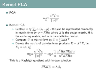
  • 10. Kernel PCA PCA: ˆ wT C w max w w 2 Kernel PCA: Replace w by i αi (xi − ”) - this can be represented compactly in matrix form by w = XH α where X is the design matrix, H is the centering matrix, and α is the coeïŹƒcient vector.
  • 11. Kernel PCA PCA: ˆ wT C w max w w 2 Kernel PCA: Replace w by i αi (xi − ”) - this can be represented compactly in matrix form by w = XH α where X is the design matrix, H is the centering matrix, and α is the coeïŹƒcient vector. ˆ ˆ 1 Compute C in matrix form as C = n XHX T
  • 12. Kernel PCA PCA: ˆ wT C w max w w 2 Kernel PCA: Replace w by i αi (xi − ”) - this can be represented compactly in matrix form by w = XH α where X is the design matrix, H is the centering matrix, and α is the coeïŹƒcient vector. ˆ ˆ 1 Compute C in matrix form as C = n XHX T Denote the matrix of pairwise inner products K = X T X , i.e. Kij = xi , xj
  • 13. Kernel PCA PCA: ˆ wT C w max w w 2 Kernel PCA: Replace w by i αi (xi − ”) - this can be represented compactly in matrix form by w = XH α where X is the design matrix, H is the centering matrix, and α is the coeïŹƒcient vector. ˆ ˆ 1 Compute C in matrix form as C = n XHX T Denote the matrix of pairwise inner products K = X T X , i.e. Kij = xi , xj ˆ wT C w 1 αT HKHKH α max = max w w 2 α n αT HKH α This is a Rayleigh quotient with known solution HKH ÎČi = λi ÎČi
  • 14. Kernel PCA Set ÎČ to be the eigenvectors of HKH , and λ the corresponding eigenvalues 1 Set α = ÎČλ− 2 Example, image super-resolution: (ïŹg: Kim et al., PAMI 2005.)
  • 15. Overview Kernel Ridge Regression Kernel PCA Spectral Clustering Kernel Covariance and Canonical Correlation Analysis Kernel Measures of Independence
  • 16. Spectral Clustering Represent similarity of images by weights on a graph Normalized cuts optimizes the ratio of the cost of a cut and the volume of each cluster k ÂŻ cut(Ai , Ai ) Ncut(A1 , . . . , Ak ) = i=1 vol(Ai )
  • 17. Spectral Clustering Represent similarity of images by weights on a graph Normalized cuts optimizes the ratio of the cost of a cut and the volume of each cluster k ÂŻ cut(Ai , Ai ) Ncut(A1 , . . . , Ak ) = i=1 vol(Ai ) Exact optimization is NP-hard, but relaxed version can be solved by ïŹnding the eigenvalues of the graph Laplacian 1 1 L = I − D − 2 AD − 2 where D is the diagonal matrix with entries equal to the row sums of similarity matrix, A.
  • 18. Spectral Clustering (continued) 1 1 Compute L = I − D − 2 AD − 2 . Map data points based on the eigenvalues of L Example, handwritten digits (0-9): (ïŹg: Xiaofei He) Cluster in mapped space using k-means
  • 19. Overview Kernel Ridge Regression Kernel PCA Spectral Clustering Kernel Covariance and Canonical Correlation Analysis Kernel Measures of Independence
  • 20. Multimodal Data A latent aspect relates data that are present in multiple modalities e.g. images and text XYZ[ _^] z M qqq MMM qqq MMM XYZ[ _^] _^] XYZ[ q x & ϕx (x) ϕy (y) x: y: “A view from Idyllwild, California, with pine trees and snow capped Marion Mountain under a blue sky.”
  • 21. Multimodal Data A latent aspect relates data that are present in multiple modalities e.g. images and text XYZ[ _^] z M qqq MMM qqq MMM XYZ[ _^] _^] XYZ[ q x & ϕx (x) ϕy (y) x: y: “A view from Idyllwild, California, with pine trees and snow capped Marion Mountain under a blue sky.” Learn kernelized projections that relate both spaces
  • 22. Kernel Covariance KPCA is maximization of auto-covariance Instead maximize cross-covariance wx Cxy wy max w ,w x y wx wy
  • 23. Kernel Covariance KPCA is maximization of auto-covariance Instead maximize cross-covariance wx Cxy wy max w ,w x y wx wy Can also be kernelized (replace wx by i αi (xi − ”x ), etc.) αT HKx HKy H ÎČ maxα,ÎČ Î±T HKx H αÎČ T HKy H ÎČ
  • 24. Kernel Covariance KPCA is maximization of auto-covariance Instead maximize cross-covariance wx Cxy wy max w ,w x y wx wy Can also be kernelized (replace wx by i αi (xi − ”x ), etc.) αT HKx HKy H ÎČ maxα,ÎČ Î±T HKx H αÎČ T HKy H ÎČ Solution is given by (generalized) eigenproblem 0 HKx HKy H α HKx H 0 α =λ HKy HKx H 0 ÎČ 0 HKy H ÎČ
  • 25. Kernel Canonical Correlation Analysis (KCCA) Alternately, maximize correlation instead of covariance T wx Cxy wy max wx ,wy T T wx Cxx wx wy Cyy wy
  • 26. Kernel Canonical Correlation Analysis (KCCA) Alternately, maximize correlation instead of covariance T wx Cxy wy max wx ,wy T T wx Cxx wx wy Cyy wy Kernelization is straightforward as before αT HKx HKy H ÎČ max α,ÎČ Î±T (HKx H )2 αÎČ T (HKy H )2 ÎČ
  • 27. KCCA (continued) Problem: If the data in either modality are linearly independent (as many dimensions as data points), there exists a projection of the data that respects any arbitrary ordering Perfect correlation can always be achieved
  • 28. KCCA (continued) Problem: If the data in either modality are linearly independent (as many dimensions as data points), there exists a projection of the data that respects any arbitrary ordering Perfect correlation can always be achieved This is even more likely when a kernel is used (e.g. Gaussian)
  • 29. KCCA (continued) Problem: If the data in either modality are linearly independent (as many dimensions as data points), there exists a projection of the data that respects any arbitrary ordering Perfect correlation can always be achieved This is even more likely when a kernel is used (e.g. Gaussian) Solution: Regularize T wx Cxy wy max wx ,wy (wx Cxx wx + Δx wx 2 ) wy Cyy wy + Δy wy T T 2 As Δx → ∞, Δx → ∞, solution approaches maximum covariance
  • 30. KCCA Algorithm Compute Kx , Ky Solve for α and ÎČ as the eigenvectors of 0 HKx HKy H α = HKy HKx H 0 ÎČ (HKx H )2 + Δx HKx H 0 α λ 2 0 (HKy H ) + Δy HKy H ÎČ
  • 31. Content Based Image Retrieval with KCCA Hardoon et al., 2004 Training data consists of images with text captions Learn embeddings of both spaces using KCCA and appropriately chosen image and text kernels Retrieval consists of ïŹnding images whose embeddings are related to the embedding of the text query
  • 32. Content Based Image Retrieval with KCCA Hardoon et al., 2004 Training data consists of images with text captions Learn embeddings of both spaces using KCCA and appropriately chosen image and text kernels Retrieval consists of ïŹnding images whose embeddings are related to the embedding of the text query A kind of multi-variate regression
  • 33. Overview Kernel Ridge Regression Kernel PCA Spectral Clustering Kernel Covariance and Canonical Correlation Analysis Kernel Measures of Independence
  • 34. Kernel Measures of Independence We know how to measure correlation in the kernelized space
  • 35. Kernel Measures of Independence We know how to measure correlation in the kernelized space Independence implies zero correlation
  • 36. Kernel Measures of Independence We know how to measure correlation in the kernelized space Independence implies zero correlation DiïŹ€erent kernels encode diïŹ€erent statistical properties of the data
  • 37. Kernel Measures of Independence We know how to measure correlation in the kernelized space Independence implies zero correlation DiïŹ€erent kernels encode diïŹ€erent statistical properties of the data Use an appropriate kernel such that zero correlation in the Hilbert space implies independence
  • 38. Example: Polynomial Kernel First degree polynomial kernel (i.e. linear) captures correlation only Second degree polynomial kernel captures all second order statistics ...
  • 39. Example: Polynomial Kernel First degree polynomial kernel (i.e. linear) captures correlation only Second degree polynomial kernel captures all second order statistics ... A Gaussian kernel can be written 2 k(xi , xj ) = e −γ xi −xj = e −γ xi ,xi e 2Îł xi ,xj e −γ xj ,xj and we can use the identity ∞ 1 i ez = z i=1 i!
  • 40. Example: Polynomial Kernel First degree polynomial kernel (i.e. linear) captures correlation only Second degree polynomial kernel captures all second order statistics ... A Gaussian kernel can be written 2 k(xi , xj ) = e −γ xi −xj = e −γ xi ,xi e 2Îł xi ,xj e −γ xj ,xj and we can use the identity ∞ 1 i ez = z i=1 i! We can view the Gaussian kernel as being related to an appropriately scaled inïŹnite dimensional polynomial kernel
  • 41. Example: Polynomial Kernel First degree polynomial kernel (i.e. linear) captures correlation only Second degree polynomial kernel captures all second order statistics ... A Gaussian kernel can be written 2 k(xi , xj ) = e −γ xi −xj = e −γ xi ,xi e 2Îł xi ,xj e −γ xj ,xj and we can use the identity ∞ 1 i ez = z i=1 i! We can view the Gaussian kernel as being related to an appropriately scaled inïŹnite dimensional polynomial kernel captures all order statistics
  • 42. Hilbert-Schmidt Independence Criterion F RKHS on X with kernel kx (x, x ), G RKHS on Y with kernel ky (y, y )
  • 43. Hilbert-Schmidt Independence Criterion F RKHS on X with kernel kx (x, x ), G RKHS on Y with kernel ky (y, y ) Covariance operator: Cxy : G → F such that f , Cxy g F = Ex,y [f (x)g(y)] − Ex [f (x)]Ey [g(y)]
  • 44. Hilbert-Schmidt Independence Criterion F RKHS on X with kernel kx (x, x ), G RKHS on Y with kernel ky (y, y ) Covariance operator: Cxy : G → F such that f , Cxy g F = Ex,y [f (x)g(y)] − Ex [f (x)]Ey [g(y)] HSIC is the Hilbert-Schmidt norm of Cxy (Fukumizu et al. 2008): 2 HSIC := Cxy HS
  • 45. Hilbert-Schmidt Independence Criterion F RKHS on X with kernel kx (x, x ), G RKHS on Y with kernel ky (y, y ) Covariance operator: Cxy : G → F such that f , Cxy g F = Ex,y [f (x)g(y)] − Ex [f (x)]Ey [g(y)] HSIC is the Hilbert-Schmidt norm of Cxy (Fukumizu et al. 2008): 2 HSIC := Cxy HS (Biased) empirical HSIC: 1 HSIC := Tr(Kx HKy H ) n2
  • 46. Hilbert-Schmidt Independence Criterion (continued) Ring-shaped density, correlation approx. zero Maximum singular vectors (functions) of Cxy Dependence witness, X 0.5 Correlation: −0.00 1.5 Correlation: −0.90 COCO: 0.14 f(x) 0 1 1 −0.5 0.5 0.5 −1 −2 0 2 g(Y) x 0 Y 0 Dependence witness, Y 0.5 −0.5 −0.5 0 −1 g(y) −0.5 −1 −1.5 −1 −0.5 0 0.5 −2 0 2 f(X) X −1 −2 0 2 y
  • 47. Hilbert-Schmidt Normalized Independence Criterion Hilbert-Schmidt Independence Criterion analogous to cross-covariance Can we construct a version analogous to correlation?
  • 48. Hilbert-Schmidt Normalized Independence Criterion Hilbert-Schmidt Independence Criterion analogous to cross-covariance Can we construct a version analogous to correlation? Simple modiïŹcation: decompose Covariance operator (Baker 1973) 1 1 Cxy = Cxx Vxy Cyy 2 2 where Vxy is the normalized cross-covariance operator (maximum singular value is bounded by 1)
  • 49. Hilbert-Schmidt Normalized Independence Criterion Hilbert-Schmidt Independence Criterion analogous to cross-covariance Can we construct a version analogous to correlation? Simple modiïŹcation: decompose Covariance operator (Baker 1973) 1 1 Cxy = Cxx Vxy Cyy 2 2 where Vxy is the normalized cross-covariance operator (maximum singular value is bounded by 1) Use norm of Vxy instead of the norm of Cxy
  • 50. Hilbert-Schmidt Normalized Independence Criterion (continued) DeïŹne the normalized independence criterion to be the Hilbert-Schmidt norm of Vxy 1 HSNIC := 2 Tr HKx H (HKx H + Δx I )−1 n HKy H (HKy H + Δy I )−1 where Δx and Δy are regularization parameters as in KCCA
  • 51. Hilbert-Schmidt Normalized Independence Criterion (continued) DeïŹne the normalized independence criterion to be the Hilbert-Schmidt norm of Vxy 1 HSNIC := 2 Tr HKx H (HKx H + Δx I )−1 n HKy H (HKy H + Δy I )−1 where Δx and Δy are regularization parameters as in KCCA If the kernels on x and y are characteristic (e.g. Gaussian kernels, see Fukumizu et al., 2008) Cxy 2 = Vxy 2 = 0 iïŹ€ x and y are independent! HS HS
  • 52. Applications of HS(N)IC Independence tests - is there anything to gain from the use of multi-modal data?
  • 53. Applications of HS(N)IC Independence tests - is there anything to gain from the use of multi-modal data? Kernel ICA
  • 54. Applications of HS(N)IC Independence tests - is there anything to gain from the use of multi-modal data? Kernel ICA Maximize dependence with respect to some model parameters Kernel target alignment (Cristianini et al., 2001)
  • 55. Applications of HS(N)IC Independence tests - is there anything to gain from the use of multi-modal data? Kernel ICA Maximize dependence with respect to some model parameters Kernel target alignment (Cristianini et al., 2001) Learning spectral clustering (Bach & Jordan, 2003) - relates kernel learning and clustering
  • 56. Applications of HS(N)IC Independence tests - is there anything to gain from the use of multi-modal data? Kernel ICA Maximize dependence with respect to some model parameters Kernel target alignment (Cristianini et al., 2001) Learning spectral clustering (Bach & Jordan, 2003) - relates kernel learning and clustering Taxonomy discovery (Blaschko & Gretton, 2008)
  • 57. Summary In this section we learned how to Do basic operations in kernel space like: Regularized least squares regression Data centering PCA
  • 58. Summary In this section we learned how to Do basic operations in kernel space like: Regularized least squares regression Data centering PCA Learn with multi-modal data Kernel Covariance KCCA
  • 59. Summary In this section we learned how to Do basic operations in kernel space like: Regularized least squares regression Data centering PCA Learn with multi-modal data Kernel Covariance KCCA Use kernels to construct statistical independence tests Use appropriate kernels to capture relevant statistics Measure dependence by norm of (normalized) covariance operator Closed form solutions requiring only kernel matrices for each modality
  • 60. Summary In this section we learned how to Do basic operations in kernel space like: Regularized least squares regression Data centering PCA Learn with multi-modal data Kernel Covariance KCCA Use kernels to construct statistical independence tests Use appropriate kernels to capture relevant statistics Measure dependence by norm of (normalized) covariance operator Closed form solutions requiring only kernel matrices for each modality Questions?
  • 61. Structured Output Learning Christoph Lampert & Matthew Blaschko Max-Planck-Institute for Biological Cybernetics Department Schölkopf: Empirical Inference TĂŒbingen, Germany Visual Geometry Group University of Oxford United Kingdom June 20, 2009
  • 62. What is Structured Output Learning? Regression maps from an input space to an output space g:X →Y
  • 63. What is Structured Output Learning? Regression maps from an input space to an output space g:X →Y In typical scenarios, Y ≡ R (regression) or Y ≡ {−1, 1} (classiïŹcation)
  • 64. What is Structured Output Learning? Regression maps from an input space to an output space g:X →Y In typical scenarios, Y ≡ R (regression) or Y ≡ {−1, 1} (classiïŹcation) Structured output learning extends this concept to more complex and interdependent output spaces
  • 65. Examples of Structured Output Problems in Computer Vision Multi-class classiïŹcation (Crammer & Singer, 2001) Hierarchical classiïŹcation (Cai & Hofmann, 2004) Segmentation of 3d scan data (Anguelov et al., 2005) Learning a CRF model for stereo vision (Li & Huttenlocher, 2008) Object localization (Blaschko & Lampert, 2008) Segmentation with a learned CRF model (Szummer et al., 2008) ... More examples at CVPR 2009
  • 66. Generalization of Regression Direct discriminative learning of g : X → Y Penalize errors for this mapping
  • 67. Generalization of Regression Direct discriminative learning of g : X → Y Penalize errors for this mapping Two basic assumptions employed Use of a compatibility function f :X ×Y →R g takes the form of a decoding function g(x) = argmax f (x, y) y
  • 68. Generalization of Regression Direct discriminative learning of g : X → Y Penalize errors for this mapping Two basic assumptions employed Use of a compatibility function f :X ×Y →R g takes the form of a decoding function g(x) = argmax f (x, y) y linear w.r.t. joint kernel f (x, y) = w, ϕ(x, y)
  • 69. Multi-Class Joint Feature Map Simple joint kernel map: deïŹne ϕy (yi ) to be the vector with 1 in place of the current class, and 0 elsewhere ϕy (yi ) = [0, . . . , 1 , . . . , 0]T kth position if yi represents a sample that is a member of class k
  • 70. Multi-Class Joint Feature Map Simple joint kernel map: deïŹne ϕy (yi ) to be the vector with 1 in place of the current class, and 0 elsewhere ϕy (yi ) = [0, . . . , 1 , . . . , 0]T kth position if yi represents a sample that is a member of class k ϕx (xi ) can result from any kernel over X : kx (xi , xj ) = ϕx (xi ), ϕx (xj )
  • 71. Multi-Class Joint Feature Map Simple joint kernel map: deïŹne ϕy (yi ) to be the vector with 1 in place of the current class, and 0 elsewhere ϕy (yi ) = [0, . . . , 1 , . . . , 0]T kth position if yi represents a sample that is a member of class k ϕx (xi ) can result from any kernel over X : kx (xi , xj ) = ϕx (xi ), ϕx (xj ) Set ϕ(xi , yi ) = ϕy (yi ) ⊗ ϕx (xi ), where ⊗ represents the Kronecker product
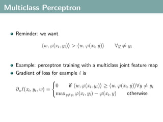
  • 72. Multiclass Perceptron Reminder: we want w, ϕ(xi , yi ) > w, ϕ(xi , y) ∀y = yi
  • 73. Multiclass Perceptron Reminder: we want w, ϕ(xi , yi ) > w, ϕ(xi , y) ∀y = yi Example: perceptron training with a multiclass joint feature map Gradient of loss for example i is ïŁ± ïŁČ0 if w, ϕ(xi , yi ) ≄ w, ϕ(xi , y) ∀y = yi ∂w (xi , yi , w) = ïŁłmaxy=y ϕ(xi , yi ) − ϕ(xi , y) otherwise i
  • 74. Perceptron Training with Multiclass Joint Feature Map (Credit: Lyndsey Pickup)
  • 75. Perceptron Training with Multiclass Joint Feature Map (Credit: Lyndsey Pickup)
  • 76. Perceptron Training with Multiclass Joint Feature Map (Credit: Lyndsey Pickup)
  • 77. Perceptron Training with Multiclass Joint Feature Map (Credit: Lyndsey Pickup)
  • 78. Perceptron Training with Multiclass Joint Feature Map (Credit: Lyndsey Pickup)
  • 79. Perceptron Training with Multiclass Joint Feature Map (Credit: Lyndsey Pickup)
  • 80. Perceptron Training with Multiclass Joint Feature Map (Credit: Lyndsey Pickup)
  • 81. Perceptron Training with Multiclass Joint Feature Map (Credit: Lyndsey Pickup)
  • 82. Perceptron Training with Multiclass Joint Feature Map (Credit: Lyndsey Pickup)
  • 83. Perceptron Training with Multiclass Joint Feature Map (Credit: Lyndsey Pickup)
  • 84. Perceptron Training with Multiclass Joint Feature Map (Credit: Lyndsey Pickup)
  • 85. Perceptron Training with Multiclass Joint Feature Map (Credit: Lyndsey Pickup)
  • 86. Perceptron Training with Multiclass Joint Feature Map (Credit: Lyndsey Pickup)
  • 87. Perceptron Training with Multiclass Joint Feature Map (Credit: Lyndsey Pickup)
  • 88. Perceptron Training with Multiclass Joint Feature Map (Credit: Lyndsey Pickup)
  • 89. Perceptron Training with Multiclass Joint Feature Map Final result (Credit: Lyndsey Pickup)
  • 90. Perceptron Training with Multiclass Joint Feature Map (Credit: Lyndsey Pickup)
  • 91. Crammer & Singer Multi-Class SVM Instead of training using a perceptron, we can enforce a large margin and do a batch convex optimization: n 1 min w 2+C Οi w 2 i=1 s.t. w, ϕ(xi , yi ) − w, ϕ(xi , y) ≄ 1 − Οi ∀y = yi
  • 92. Crammer & Singer Multi-Class SVM Instead of training using a perceptron, we can enforce a large margin and do a batch convex optimization: n 1 min w 2+C Οi w 2 i=1 s.t. w, ϕ(xi , yi ) − w, ϕ(xi , y) ≄ 1 − Οi ∀y = yi Can also be written only in terms of kernels w= αxy ϕ(x, y) x y Can use a joint kernel k :X ×Y ×X ×Y →R k(xi , yi , xj , yj ) = ϕ(xi , yi ), ϕ(xj , yj )
  • 93. Structured Output Support Vector Machines (SO-SVM) Frame structured prediction as a multiclass problem predict a single element of Y and pay a penalty for mistakes
  • 94. Structured Output Support Vector Machines (SO-SVM) Frame structured prediction as a multiclass problem predict a single element of Y and pay a penalty for mistakes Not all errors are created equally e.g. in an HMM making only one mistake in a sequence should be penalized less than making 50 mistakes
  • 95. Structured Output Support Vector Machines (SO-SVM) Frame structured prediction as a multiclass problem predict a single element of Y and pay a penalty for mistakes Not all errors are created equally e.g. in an HMM making only one mistake in a sequence should be penalized less than making 50 mistakes Pay a loss proportional to the diïŹ€erence between true and predicted error (task dependent) ∆(yi , y)
  • 96. Margin Rescaling Variant: Margin-Rescaled Joint-Kernel SVM for output space Y (Tsochantaridis et al., 2005) Idea: some wrong labels are worse than others: loss ∆(yi , y) Solve n 2 min w w +C Οi i=1 s.t. w, ϕ(xi , yi ) − w, ϕ(xi , y) ≄ ∆(yi , y) − Οi ∀y ∈ Y {yi } Classify new samples using g : X → Y: g(x) = argmax w, ϕ(x, y) y∈Y
  • 97. Margin Rescaling Variant: Margin-Rescaled Joint-Kernel SVM for output space Y (Tsochantaridis et al., 2005) Idea: some wrong labels are worse than others: loss ∆(yi , y) Solve n 2 min w w +C Οi i=1 s.t. w, ϕ(xi , yi ) − w, ϕ(xi , y) ≄ ∆(yi , y) − Οi ∀y ∈ Y {yi } Classify new samples using g : X → Y: g(x) = argmax w, ϕ(x, y) y∈Y Another variant is slack rescaling (see Tsochantaridis et al., 2005)
  • 98. Label Sequence Learning For, e.g., handwritten character recognition, it may be useful to include a temporal model in addition to learning each character individually As a simple example take an HMM
  • 99. Label Sequence Learning For, e.g., handwritten character recognition, it may be useful to include a temporal model in addition to learning each character individually As a simple example take an HMM We need to model emission probabilities and transition probabilities Learn these discriminatively
  • 100. A Joint Kernel Map for Label Sequence Learning Emissions (blue)
  • 101. A Joint Kernel Map for Label Sequence Learning Emissions (blue) fe (xi , yi ) = we , ϕe (xi , yi )
  • 102. A Joint Kernel Map for Label Sequence Learning Emissions (blue) fe (xi , yi ) = we , ϕe (xi , yi ) Can simply use the multi-class joint feature map for ϕe
  • 103. A Joint Kernel Map for Label Sequence Learning Emissions (blue) fe (xi , yi ) = we , ϕe (xi , yi ) Can simply use the multi-class joint feature map for ϕe Transitions (green)
  • 104. A Joint Kernel Map for Label Sequence Learning Emissions (blue) fe (xi , yi ) = we , ϕe (xi , yi ) Can simply use the multi-class joint feature map for ϕe Transitions (green) ft (xi , yi ) = wt , ϕt (yi , yi+1 ) Can use ϕt (yi , yi+1 ) = ϕy (yi ) ⊗ ϕy (yi+1 )
  • 105. A Joint Kernel Map for Label Sequence Learning (continued) p(x, y) ∝ e fe (xi ,yi ) e ft (yi ,yi+1 ) for an HMM i i
  • 106. A Joint Kernel Map for Label Sequence Learning (continued) p(x, y) ∝ e fe (xi ,yi ) e ft (yi ,yi+1 ) for an HMM i i f (x, y) = fe (xi , yi ) + ft (yi , yi+1 ) i i = we , ϕe (xi , yi ) + wt , ϕt (yi , yi+1 ) i i
  • 107. Constraint Generation n 2 min w +C Οi w i=1 s.t. w, ϕ(xi , yi ) − w, ϕ(xi , y) ≄ ∆(yi , y) − Οi ∀y ∈ Y {yi }
  • 108. Constraint Generation n 2 min w +C Οi w i=1 s.t. w, ϕ(xi , yi ) − w, ϕ(xi , y) ≄ ∆(yi , y) − Οi ∀y ∈ Y {yi } Initialize constraint set to be empty Iterate until convergence: Solve optimization using current constraint set Add maximially violated constraint for current solution
  • 109. Constraint Generation with the Viterbi Algorithm To ïŹnd the maximially violated constraint, we need to maximize w.r.t. y w, ϕ(xi , y) + ∆(yi , y)
  • 110. Constraint Generation with the Viterbi Algorithm To ïŹnd the maximially violated constraint, we need to maximize w.r.t. y w, ϕ(xi , y) + ∆(yi , y) For arbitrary output spaces, we would need to iterate over all elements in Y
  • 111. Constraint Generation with the Viterbi Algorithm To ïŹnd the maximially violated constraint, we need to maximize w.r.t. y w, ϕ(xi , y) + ∆(yi , y) For arbitrary output spaces, we would need to iterate over all elements in Y For HMMs, maxy w, ϕ(xi , y) can be found using the Viterbi algorithm
  • 112. Constraint Generation with the Viterbi Algorithm To ïŹnd the maximially violated constraint, we need to maximize w.r.t. y w, ϕ(xi , y) + ∆(yi , y) For arbitrary output spaces, we would need to iterate over all elements in Y For HMMs, maxy w, ϕ(xi , y) can be found using the Viterbi algorithm It is a simple modiïŹcation of this procedure to incorporate ∆(yi , y) (Tsochantaridis et al., 2004)
  • 113. Discriminative Training of Object Localization Structured output learning is not restricted to outputs speciïŹed by graphical models
  • 114. Discriminative Training of Object Localization Structured output learning is not restricted to outputs speciïŹed by graphical models We can formulate object localization as a regression from an image to a bounding box g:X →Y X is the space of all images Y is the space of all bounding boxes
  • 115. Joint Kernel between Images and Boxes: Restriction Kernel Note: x |y (the image restricted to the box region) is again an image. Compare two images with boxes by comparing the images within the boxes: kjoint ((x, y), (x , y ) ) = kimage (x |y , x |y , ) Any common image kernel is applicable: linear on cluster histograms: k(h, h ) = i hi hi , 1 (h −h )2 χ2 -kernel: kχ2 (h, h ) = exp − Îł i hii +hi i pyramid matching kernel, ... The resulting joint kernel is positive deïŹnite.
  • 116. Restriction Kernel: Examples kjoint , =k , is large. kjoint , =k , is small. kjoint , =k , could also be large. Note: This behaves diïŹ€erently from the common tensor products kjoint ( (x, y), (x , y ) ) = k(x, x )k(y, y )) !
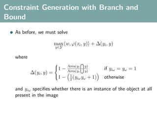
  • 117. Constraint Generation with Branch and Bound As before, we must solve max w, ϕ(xi , y) + ∆(yi , y) y∈Y where ïŁ± ïŁČ1 − Area(yi y) if yiω = yω = 1 Area(yi y) ∆(yi , y) = 1 ïŁł1 − (y y + 1) otherwise 2 iω ω and yiω speciïŹes whether there is an instance of the object at all present in the image
  • 118. Constraint Generation with Branch and Bound As before, we must solve max w, ϕ(xi , y) + ∆(yi , y) y∈Y where ïŁ± ïŁČ1 − Area(yi y) if yiω = yω = 1 Area(yi y) ∆(yi , y) = 1 ïŁł1 − (y y + 1) otherwise 2 iω ω and yiω speciïŹes whether there is an instance of the object at all present in the image Solution: use branch-and-bound over the space of all rectangles in the image (Blaschko & Lampert, 2008)
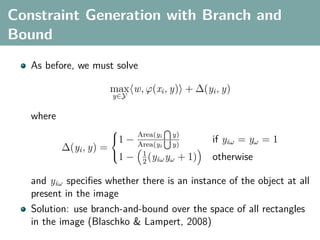
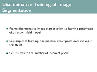
  • 119. Discriminative Training of Image Segmentation Frame discriminative image segmentation as learning parameters of a random ïŹeld model
  • 120. Discriminative Training of Image Segmentation Frame discriminative image segmentation as learning parameters of a random ïŹeld model Like sequence learning, the problem decomposes over cliques in the graph
  • 121. Discriminative Training of Image Segmentation Frame discriminative image segmentation as learning parameters of a random ïŹeld model Like sequence learning, the problem decomposes over cliques in the graph Set the loss to the number of incorrect pixels
  • 122. Constraint Generation with Graph Cuts As the graph is loopy, we cannot use Viterbi
  • 123. Constraint Generation with Graph Cuts As the graph is loopy, we cannot use Viterbi Loopy belief propagation is approximate and can lead to poor learning performance for structured output learning of graphical models (Finley & Joachims, 2008)
  • 124. Constraint Generation with Graph Cuts As the graph is loopy, we cannot use Viterbi Loopy belief propagation is approximate and can lead to poor learning performance for structured output learning of graphical models (Finley & Joachims, 2008) Solution: use graph cuts (Szummer et al., 2008) ∆(yi , y) can be easily incorporated into the energy function
  • 125. Summary of Structured Output Learning Structured output learning is the prediction of items in complex and interdependent output spaces
  • 126. Summary of Structured Output Learning Structured output learning is the prediction of items in complex and interdependent output spaces We can train regressors into these spaces using a generalization of the support vector machine
  • 127. Summary of Structured Output Learning Structured output learning is the prediction of items in complex and interdependent output spaces We can train regressors into these spaces using a generalization of the support vector machine We have shown examples for Label sequence learning with Viterbi Object localization with branch and bound Image segmentation with graph cuts
  • 128. Summary of Structured Output Learning Structured output learning is the prediction of items in complex and interdependent output spaces We can train regressors into these spaces using a generalization of the support vector machine We have shown examples for Label sequence learning with Viterbi Object localization with branch and bound Image segmentation with graph cuts Questions?