The Graph slide the Data Structures course include:
1. Definition of graph
2. Component of graph
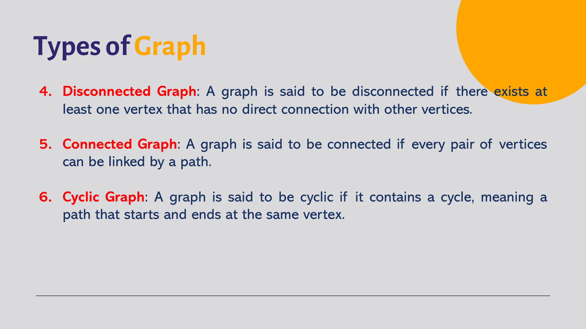
3. Types of graph
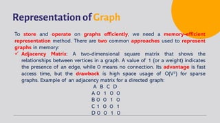
4. Representation of graph
5. Basic operation of graph
6. Vertex insertion operation
7. Edge insertion operation
8. Vertex deletion operation
9. Edge deletion operation
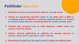
10. Pathfinder operation
11. Traversal of graph
12. Breadth-first search
13. Depth-first search
14. Algoritma of graph
15. Djikstra algorithm
16. Prim algorithm
17. Kruskal algorithm
18. Bellman-ford algorithm
19. Floyd-warshall algorithm
20. Application of graf