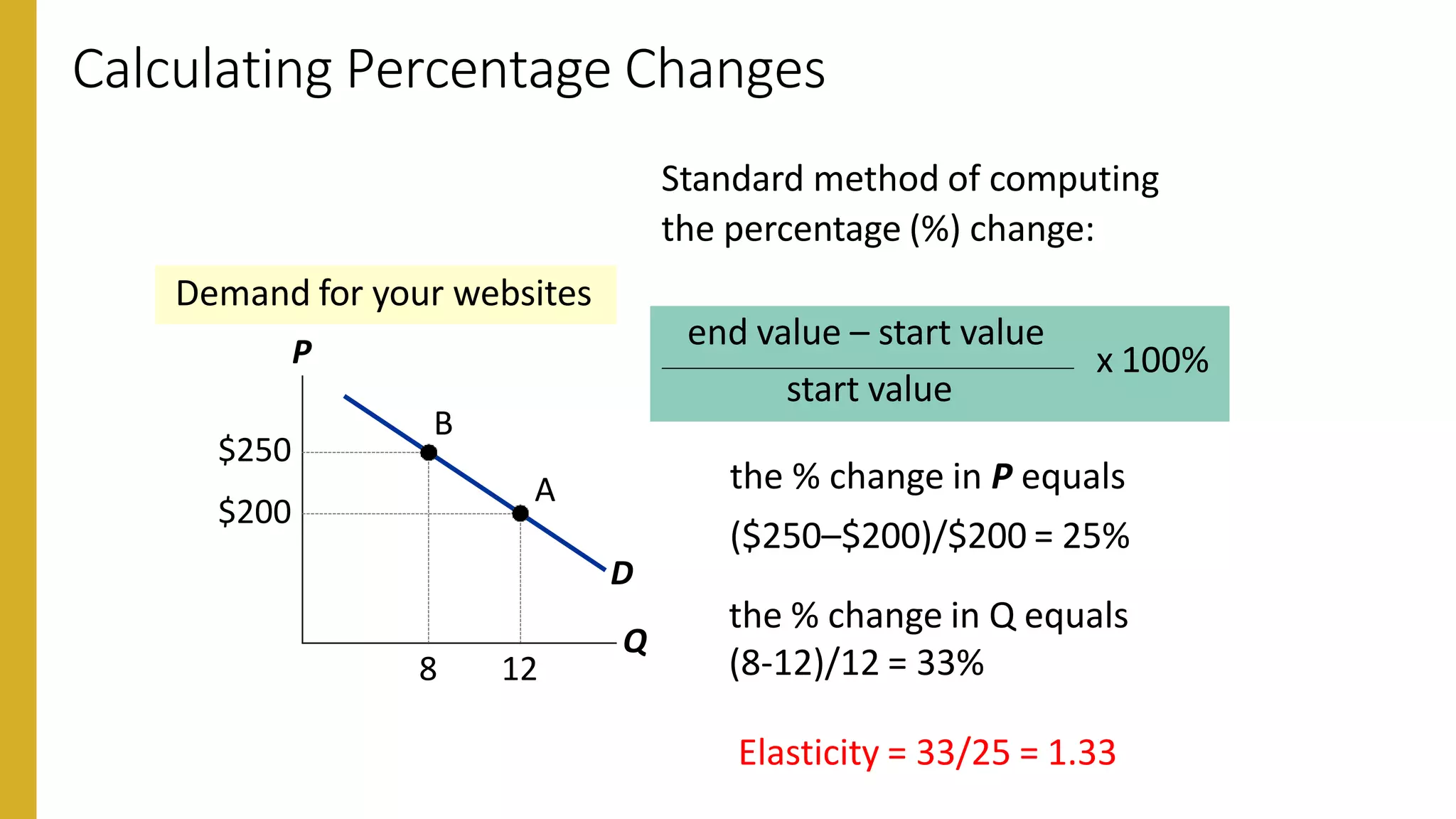
elasticityanditsapplication-220721180141-8959a8ed.pptx

Elasticity and its Application
Credit
N. Gregory Mankiw

Contents
What is elasticity? What kinds of issues can elasticity help us understand?
What is the Price Elasticity of Demand (PED)?
How is it related to the demand curve?
How is it related to revenue & expenditure?
What is the Price Elasticity of Supply?
How is it related to the supply curve?
What are the income and Cross-price Elasticities of Demand?

A scenario…
 You design websites for local businesses.
 You charge $200 per website, and currently sell 12 websites per month.
 Your costs are rising (including the opportunity cost of your time), so you consider
raising the price to $250.
 The law of demand says that you won’t sell as many websites if you raise your
price.
 How many fewer websites? How much will your revenue fall, or might it increase?

Elasticity
Basic idea:
 Elasticity measures how much one variable responds to changes in another
variable.
 One type of elasticity measures how much demand for your websites will fall if
you raise your price.
Definition:
 Elasticity is a numerical measure of the responsiveness of quantity demanded
(Qd) or quantity supplied (Qs) to one of its determinants.

Price Elasticity of Demand
• Price elasticity of demand measures how much Qd responds to
a change in P.
 Loosely speaking, it measures the price-sensitivity of
buyers’ demand.
Price Elasticity
of Demand
=
Percentage change in Qd
Percentage change in P

Price elasticity
of demand equals
P
Q
D
Q
P2
P1
Q
2 1
P rises by 10%
Q falls by 15%
15%
10%
= 1.5
Price Elasticity
of Demand
=
Example:

 Along a D curve, P and Q move in
opposite directions, which would make
price elasticity negative.
 We will drop the minus sign and report
all price elasticities as positive
numbers.
P
Q
D
Q2
P2
P1
Q1
Price elasticity
of demand
=

Calculating Percentage Changes
P
Q
D
$250
$200
8 12
B
A
Demand for your websites
Standard method of computing
the percentage (%) change:
end value – start value
start value
x 100%
the % change in P equals
($250–$200)/$200 = 25%
Elasticity = 33/25 = 1.33
the % change in Q equals
(8-12)/12 = 33%

P
Q
D
$250
$200
8 12
B
A
Demand for your websites
Problem:
The standard method gives different answers
depending on where you start.
From A to B,
P rises 25%, Q falls 33%,
elasticity = 33/25 = 1.33
From B to A,
P falls 20%, Q rises 50%, elasticity
= 50/20 = 2.50

• So, we instead use the midpoint method:
end value – start value
midpoint
x 100%
 The midpoint is the number halfway between the start and
end values, the average of those values.
 It doesn’t matter which value you use as the start and which
as the end—you get the same answer either way!

 Using the midpoint method, the % change
in P equals
$250 – $200
$225
x 100% = 22.2%
 The % change in Q equals
12 – 8
10
x 100% = 40.0%
 The price elasticity of demand equals
40/22.2 = 1.8

Class Exercise: Calculate an elasticity
 Use the following information
to calculate the price elasticity
of demand for hotel rooms:
if P = $70, Qd = 5000
if P = $90, Qd = 3000
Use midpoint method to calculate.
Answers
% change in Qd
(5000 – 3000)/4000 = 50%
% change in P
($90 – $70)/$80 = 25%
The price elasticity of demand equals
50%
25%
= 2.0

What Determines Price Elasticity?
To learn the determinants of price elasticity, we look at a series of examples.
Each compares two common goods.
In each example:
• Suppose the prices of both goods rise by 20%.
• The good for which Qd falls the most (in percent) has the highest price elasticity of
demand.
Which good is it? Why?
• What lesson does the example teach us about the determinants of the price elasticity
of demand?

EXAMPLE 1: Dosa vs. Nihari
 The prices of both of these goods rise by 20%.
For which good does Qd drop the most? Why?
• Dosa has close substitutes (e.g., Vada Pav, Paratha, Idli, Upma, Samosa etc.), so
buyers can easily switch if the price rises.
• Nihari has no close substitutes, so consumers would probably not buy much
less if its price rises.
 Lesson: Price elasticity is higher when close substitutes are available.

EXAMPLE 2: “Tata Indica” vs. “Motorbike”
 The prices of both goods rise by 20%.
• For a narrowly defined good such as Tata Indica, there are many substitutes
(Maruti Suzuki, Hyundai, Chevrolet, Renault etc.).
• There are fewer substitutes available for broadly defined goods.
(There aren’t too many substitutes for Motorbike.)
 Lesson: Price elasticity is higher for narrowly defined goods than for
broadly defined ones.

EXAMPLE 3: Insulin vs. Andaman Cruise
 The prices of both of these goods rise by 20%.
• To millions of diabetics, insulin is a necessity. A rise in its price would cause
little or no decrease in demand.
• A cruise is a luxury. If the price rises, some people will forego it.
 Lesson: Price elasticity is higher for luxuries than for necessities.

EXAMPLE 4: Petrol price in the Short Run vs. Petrol price
in the Long Run
 The price of petrol rises 20%.
 Does Qd drop more in the short run or the long run? Why?
• There’s not much people can do in the short run, other than ride the bus or
carpool.
• In the long run, people can buy smaller cars or live closer to where they work.
 Lesson: Price elasticity is higher in the long run than the short run.

The Determinants of Price Elasticity: A Summary
The price elasticity of demand depends on:
1. The extent to which close substitutes are available
2. Whether the good is a necessity or a luxury
3. How broadly or narrowly the good is defined
4. The time horizon—elasticity is higher in the long run than the short run

The Variety of Demand Curves
The price elasticity of demand is closely related to the slope of the demand curve.
 Rule of thumb:
• The flatter the curve, the bigger the elasticity.
• The steeper the curve, the smaller the elasticity.
 Five different classifications of D curves.… Economists classify demand curves
according to their elasticity. The next five slides present the five different
classifications, from least to most elastic.

Q1
P1
D
“Perfectly Inelastic Demand” (one extreme case)
P
Q
P2
P falls
by 10%
Q changes
by 0%
% change in Q 0%
% change in P 10%
= 0
Price elasticity
of demand
= =
Consumers’
price sensitivity:
none
D curve:
vertical
Elasticity:
0

D
“Inelastic Demand”
P
Q
Q Q
1 2
P1
P2
Q rises less than 10%
< 10%
10%
< 1
Price elasticity
of demand
=
% change in Q
% change in P
=
P falls by 10%
Consumers’
price sensitivity:
relatively low
D curve:
relatively steep
Elasticity:
< 1

D
“Unit Elastic Demand”
P
Q
Q1 Q2
P1
P2
Q rises by 10%
10%
10%
= 1
Price elasticity
of demand
=
% change in Q
% change in P
=
P falls by 10%
Consumers’
price sensitivity:
intermediate
Elasticity:
1
D curve:
intermediate slope

D
“Elastic Demand”
P
Q
Q
P1
Q
1 2
P2
Q rises more than 10%
> 10%
10%
> 1
Price elasticity
of demand
=
% change in Q
% change in P
=
P falls by 10%
Consumers’
price sensitivity:
relatively high
D curve:
relatively flat
Elasticity:
> 1

D
“Perfectly Elastic Demand” (the other extreme)
P
Q
P2 = P1
Q
P changes by 0%
Q changes by any %
% change in Q any %
% change in P 0%
= infinity
Q
1 2
Consumers’
price sensitivity:
extreme
D curve:
horizontal
Elasticity:
infinity
Price elasticity
of demand
= =

Elasticity of a Linear Demand Curve
The slope of a linear demand curve
is constant, but its elasticity is not.
P
Q
$30
20
10
$0
0 20 40 60
40%
E =
200%
= 5.0
67%
E =
67%
= 1.0
40%
E = = 0.2
200%
 Calculations of percentage changes use the midpoint
method. (This is why the increase from Q=0 to Q=20 is
200% rather than infinity.)
 As you move down a linear demand curve, the slope (the
ratio of the absolute change in P to that in Q) remains
constant:
 From the point (0, $30) to the point (20, $20), the
“rise” equals -$10, the “run” equals +20, so the
slope equals -1/2 or -0.5.
 From the point (40, $10) to the point (60, $0), the
“rise” again equals -$10, the “run” equals +20, and
the slope again equals -0.5.
 However, the percentage changes in these variables do
not remain constant, as shown by the different colored
elasticity calculations.
 The lesson here is that elasticity falls as you move
downward & rightward along a linear demand curve.

Price Elasticity and Total Revenue
 If you raise your price from $200 to $250, would your revenue rise or fall?
Revenue = P x Q
 A price increase has two effects on revenue:
1. Higher P means more revenue on each unit you sell.
2. But you sell fewer units (lower Q), due to law of demand.
 Which of these two effects is bigger?
It depends on the price elasticity of demand.

• If demand is elastic, then
price elasticity of demand > 1
% change in Q > % change in P
• The fall in revenue from lower Q is greater than the increase in revenue
from higher P, so revenue falls.
Revenue = P x Q
Price Elasticity
of Demand
=
Percentage change in Q

Elastic demand
(elasticity = 1.8)
P
Q
D
$200
12
If P = $200,
Q = 12 and revenue =
$2400.
When D is elastic, a price
increase causes revenue to
fall.
$250
8
If P = $250,
Q = 8 and
revenue = $2000.
lost revenue
due to lower Q
increased revenue
due to higher P
Demand for
your websites

 If demand is inelastic, then
price elasticity of demand < 1
% change in Q < % change in P
 The fall in revenue from lower Q is smaller than the increase in revenue from higher P, so
revenue rises.
 In our example, suppose that Q only falls to 10 (instead of 8) when you raise your price to $250.
Revenue = P x Q
Price elasticity
of demand
=
Percentage change in Q

Now, demand is inelastic:
elasticity = 0.82
P
Q
D
If P = $250,
Q = 10 and
revenue = $2500.
$200
When D is inelastic, a price
increase causes revenue to
rise.
12
If P = $200,
Q = 12 and revenue =
$2400. $250
10
lost revenue
due to lower Q
increased revenue
due to higher P
Demand for your
websites

Class Exercise: Elasticity and Expenditure/Revenue
Question:
As a result of a fare war, the price of a luxury cruise
falls 20%.
Does luxury cruise companies’ total revenue rise or
fall?
Answers:
 Revenue = P x Q
 The fall in P reduces revenue, but Q increases,
which increases revenue. Which effect is bigger?
 Since demand is elastic, Q will increase more than
20%, so revenue rises.
Question:
Pharmacies raise the price of insulin by
10%.
Does total expenditure on insulin rise or
fall?
Answers:
Expenditure = P x Q
Since demand is inelastic, Q will fall less
than 10%, so expenditure rises.

Does Drug Interdiction Increase or Decrease Drug-Related
Crime?
 One side effect of illegal drug use is crime: Users often turn to crime to
finance their habit.
 We examine two policies designed to reduce illegal drug use and see
what effects they have on drug-related crime.
 For simplicity, we assume the total dollar value of drug-related crime
equals total expenditure on drugs.
 Demand for illegal drugs is inelastic, due to addiction issues.

D1
Policy 1: Interdiction
Price of
Drugs
Quantity
of Drugs
S1
S2
P1
P2
Q2 Q1
Interdiction reduces the
supply of drugs.
Since demand for drugs is
inelastic, P rises
proportionally more than
Q falls.
Result:
An increase in total
spending on drugs, and in
drug-related crime.
New value of drug-related crime
Initial value of
drug-related
crime

Policy 2: Education
Price of
Drugs
Quantity
of Drugs
S
Q1
D2 D1
P1
P2
Q2
Education reduces the
demand for drugs.
P and Q fall.
Result:
A decrease in total spending
on drugs, and in drug-related
crime.
Initial value
of drug-
related crime
New value of drug-related
crime

Price Elasticity of Supply
• Price Elasticity of Supply measures how much Qs responds to a
change in P.
 Loosely speaking, it measures sellers’ price-sensitivity.
 Again, use the midpoint method to compute the percentage
changes.
Price elasticity of
supply
=
Percentage change in Qs

Q1 Q2
Price Elasticity of Supply
Price elasticity
of supply equals
P
Q
S
P2
P1
P rises by 8%
Q rises by 16%
16%
8%
= 2.0
Price elasticity of
supply
=
Percentage change in Qs
Example:

The Variety of Supply Curves
The slope of the supply curve is closely related to price elasticity of
supply.
Rule of thumb:
 The flatter the curve, the bigger the elasticity.
 The steeper the curve, the smaller the elasticity.
 Five different classifications…

S
“Perfectly Inelastic” (one extreme)
P
Q
Q1
P2
P1
Q changes by 0%
0%
10%
= 0
Price elasticity
of supply
=
% change in Q
% change in P
=
P rises by 10%
Sellers’
price sensitivity:
none
S curve:
vertical
Elasticity:
0

S
“Inelastic”
P
Q
Q
P1
Q
1 2
P2
Q rises less than 10%
< 10%
10%
< 1
Price elasticity
of supply
=
% change in Q
% change in P
=
P rises by 10%
Sellers’
price sensitivity:
relatively low
S curve:
relatively steep
Elasticity:
< 1

S
“Unit Elastic”
P
Q
Q1 Q2
P2
P1
Q rises by 10%
10%
10%
= 1
Price elasticity
of supply
=
% change in Q
% change in P
=
P rises by 10%
Sellers’
price sensitivity:
intermediate
S curve:
intermediate slope
Elasticity:
= 1

S
“Elastic”
P
Q
Q
P2
P1
Q
1 2
Q rises more than 10%
> 10%
10%
> 1
Price elasticity
of supply
=
% change in Q
% change in P
=
P rises by 10%
Sellers’
price sensitivity:
relatively high
S curve:
relatively flat
Elasticity:
> 1

S
“Perfectly Elastic” (the other extreme)
P
Q
P2 = P1
Q
P changes by 0%
Q changes by any %
any %
0%
= infinity
Price elasticity
of supply
=
% change in Q
% change in P
=
Q
1 2
Sellers’ price sensitivity:
extreme
S curve:
horizontal
Elasticity:
infinity

The Determinants of Supply Elasticity
1. The more easily sellers can change the quantity they produce, the
greater the price elasticity of supply.
• Example: Supply of beachfront property is harder to vary and thus less elastic than
supply of new cars.
2. For many goods, price elasticity of supply is greater in the long run than
in the short run, because firms can build new factories, or new firms may
be able to enter the market.

Elasticity and Changes in Equilibrium
 The supply of beachfront property is inelastic. The supply of new cars
is elastic.
 Suppose population growth causes demand for both goods to double
(at each price, Qd doubles).
1. For which product will P change the most?
2. For which product will Q change the most?

Beachfront property
(inelastic supply)
P
Q
S
Q1 Q2
P1 A
D1 D2
When supply is inelastic,
an increase in demand has
a bigger impact on price
than on quantity.
B
P2
Answers

New cars
(elastic supply):
Q
S
Q1
P2
P1
A
P
D1 D2
When supply is elastic,
an increase in demand
has a bigger impact on
quantity than on price.
Q2
B
Answers

S
How the Price Elasticity of Supply Can Vary
Supply often becomes
less elastic as Q rises,
due to capacity limits.
P
Q
$15
12
500 525
4
$3
100 200
elasticity
> 1
elasticity
< 1

Other Elasticities
Income Elasticity of Demand measures the response of Qd to a change in
consumer income
Income elasticity
of demand
=
Percent change in Qd
Percent change in income
 Recall: An increase in income causes an increase in demand for a normal
good.
 Hence, for normal goods, income elasticity > 0.
 For inferior goods, income elasticity < 0.

Other Elasticities
Cross-price Elasticity of Demand:
measures the response of demand for one good to changes in the price of
another good.
Cross-price Elasticity
of Demand
=
% change in Qd for good 1
% change in price of good 2
 For substitutes, cross-price elasticity > 0
 (e.g., an increase in price of mutton causes an increase in demand for
chicken)
 For complements, cross-price elasticity < 0
 (e.g., an increase in price of computers causes decrease in demand for
software)

 Elasticity measures the responsiveness of Qd or Qs to one of its determinants.
 Price elasticity of demand equals percentage change in Qd divided by percentage change in P. When it’s
less than one, demand is “inelastic.” When greater than one, demand is “elastic.”
 When demand is inelastic, total revenue rises when price rises. When demand is elastic, total revenue
falls when price rises.
 Demand is less elastic: in the short run; for necessities; for broadly defined goods; and for goods with few
close substitutes.
 Price elasticity of supply equals percentage change in Qs divided by percentage change in P. When it’s less
than one, supply is “inelastic.” When greater than one, supply is “elastic.”
 Price elasticity of supply is greater in the long run than in the short run.
 The income elasticity of demand (YED) measures how much quantity demanded responds to changes in
buyers’ incomes.
 The cross-price elasticity of demand (XED) measures how much demand for one good responds to
changes in the price of another good.
Summary

Calculating PED
Good 𝑷𝟎 𝑸𝟎 𝑷𝟏 𝑸𝟏
X 10 100 12 98
Y 10 100 12 80
Z 10 100 12 56
o in P o in Qd %∆ in Qd %∆ in P PED Elasticity
2 2 -2 20 0.1 <1
2 20 -20 20 1 =1
2 44 -44 20 2.2 >1

Types of Elasticity
Price Elasticity of
Demand (PED)
Perfectly Elastic
Elastic
Unitary Elastic
Inelastic
Perfectly Inelastic
Cross Elasticity of
Demand (XED)
Substitute Good
Complimentary
Good
Income Elasticity
of Demand (YED)
Normal Good
Inferior Good
Price Elasticity of
Supply (PES)
Perfectly Elastic
Elastic
Unitary Elastic
Inelastic
Perfectly Inelastic

elasticityanditsapplication-220721180141-8959a8ed.pptx

More Related Content

Similar to elasticityanditsapplication-220721180141-8959a8ed.pptx

More from sadiqfarhan2

Recently uploaded

elasticityanditsapplication-220721180141-8959a8ed.pptx