[FLOLAC'14][scm] Functional Programming Using Haskell

Introduction to Functional Programming
Using Haskell
Shin-Cheng Mu
Acadmia Sinica
FLOLAC 2014
1 / 85

A Quick Introduction to Haskell
• We will be using the Glasgow Haskell Compiler (GHC).
• A Haskell compiler written in Haskell, with an interpreter that
both interprets and runs compiled code.
• Installation: the Haskell Platform:
http://hackage.haskell.org/platform/
2 / 85

Function Definition
• A function definition consists of a type declaration, and the
definition of its body:
square :: Int → Int
square x = x × x ,
smaller :: Int → Int → Int
smaller x y = if x ≤ y then x else y .
• The GHCi interpreter evaluates expressions in the loaded
context:
? square 3768
14197824
? square (smaller 5 (3 + 4))
25
3 / 85

Evaluation
One possible sequence of evaluating (simplifying, or reducing)
square (3 + 4):
square (3 + 4)
4 / 85

Evaluation
square (3 + 4):
square (3 + 4)
= { deﬁnition of + }
square 7
4 / 85

Evaluation
square (3 + 4):
square (3 + 4)
square 7
= { deﬁnition of square }
7 × 7
4 / 85

Evaluation
square (3 + 4):
square (3 + 4)
square 7
7 × 7
= { deﬁnition of × }
49 .
4 / 85

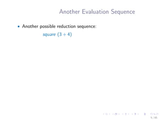
Another Evaluation Sequence
• Another possible reduction sequence:
square (3 + 4)
5 / 85

square (3 + 4)
(3 + 4) × (3 + 4)
5 / 85

square (3 + 4)
(3 + 4) × (3 + 4)
7 × (3 + 4)
5 / 85

square (3 + 4)
(3 + 4) × (3 + 4)
7 × (3 + 4)
7 × 7
5 / 85

square (3 + 4)
(3 + 4) × (3 + 4)
7 × (3 + 4)
7 × 7
= { definition of × }
49 .
• In this sequence the rule for square is applied first. The final
result stays the same.
• Do different evaluations orders always yield the same thing?
5 / 85

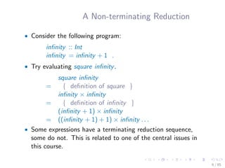
A Non-terminating Reduction
• Consider the following program:
infinity :: Int
infinity = infinity + 1 .
• Try evaluating square infinity.
square infinity
infinity × infinity
= { definition of infinity }
(infinity + 1) × infinity
= ((infinity + 1) + 1) × infinity . . .
• Some expressions have a terminating reduction sequence,
some do not. This is related to one of the central issues in
this course.
6 / 85

And, a Terminating Reduction
• In the previous case, the reduction does not terminate
because, by rule, to evaluate x + y we have to know what x is.
• Consider the following program:
three :: Int → Int
three x = 3 .
• Try evaluating three inﬁnity.
7 / 85

And, a Terminating Reduction
• If we start with simplifying three:
three infinity
= { definition of three }
3 .
• It terminates because three x need not know what x is.
• Haskell uses a peculiar reduction strategy called lazy
evaluation that evaluates an expression only when it really
needs to. It allows more program to terminate
• (while causing lots of other troubles for some people).
• We will not go into this feature in this course. For now, it is
sufficient to know
• that some expression terminate, some do not, and
• it is in general good to know that an expression may terminate.
8 / 85

Mathematical Functions
• Mathematically, a function is a mapping between arguments
and results.
• A function f :: A → B maps each element in A to a unique
element in B.
• In contrast, C “functions” are not mathematical functions:
• int y = 1; int f (x:int) { return ((y++) * x); }
• Functions in Haskell have no such side-eﬀects:
(unconstrained) assignments, IO, etc.
• Why removing these useful features? We will talk about that
later in this course.
9 / 85

Curried Functions
• Consider again the function smaller:
smaller x y = if x ≤ y then x else y
• We sometimes informally call it a function “taking two
arguments”.
• Usage: smaller 3 4.
• Strictly speaking, however, smaller is a function returning a
function. The type should be bracketed as Int → (Int → Int).
10 / 85

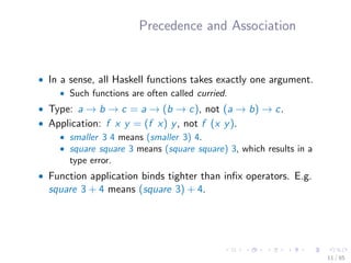
Precedence and Association
• In a sense, all Haskell functions takes exactly one argument.
• Such functions are often called curried.
• Type: a → b → c = a → (b → c), not (a → b) → c.
• Application: f x y = (f x) y, not f (x y).
• smaller 3 4 means (smaller 3) 4.
• square square 3 means (square square) 3, which results in a
type error.
• Function application binds tighter than inﬁx operators. E.g.
square 3 + 4 means (square 3) + 4.
11 / 85

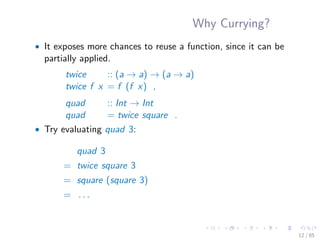
Why Currying?
• It exposes more chances to reuse a function, since it can be
partially applied.
twice :: (a → a) → (a → a)
twice f x = f (f x) ,
quad :: Int → Int
quad = twice square .
• Try evaluating quad 3:
quad 3
= twice square 3
= square (square 3)
= . . .
12 / 85

Sectioning
• Inﬁx operators are curried too. The operator (+) may have
type Int → Int → Int.
• Inﬁx operator can be partially applied too.
(x ⊕) y = x ⊕ y ,
(⊕ y) x = x ⊕ y .
• (1 +) :: Int → Int increments its argument by one.
• (1.0 /) :: Float → Float is the “reciprocal” function.
• (/ 2.0) :: Float → Float is the “halving” function.
13 / 85

Infix and Prefix
• To use an infix operator in prefix position, surrounded it in
parentheses. For example, (+) 3 4 is equivalent to 3 + 4.
• Surround an ordinary function by back-quotes (not quotes!)
to put it in infix position. E.g. 3 ‘mod‘ 4 is the same as
mod 3 4.
14 / 85

Function Composition
• Functions composition:
(·) :: (b → c) → (a → b) → (a → c)
(f · g) x = f (g x) .
• E.g. another way to write quad:
quad :: Int → Int
quad = square · square .
• Some important properties:
• id · f = f = f · id, where id x = x.
• (f · g) · h = f · (g · h).
15 / 85

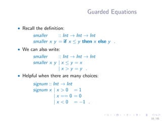
Guarded Equations
• Recall the deﬁnition:
smaller x y = if x ≤ y then x else y .
• We can also write:
smaller x y | x ≤ y = x
| x > y = y .
• Helpful when there are many choices:
signum :: Int → Int
signum x | x > 0 = 1
| x == 0 = 0
| x < 0 = −1 .
16 / 85

λ Expressions
• Since functions are ﬁrst-class constructs, we can also
construct functions in expressions.
• A λ expression denotes an anonymous function.
• λx → e: a function with argument x and body e.
• λx → λy → e abbreviates to λx y → e.
• In ASCII, we write λ as
• Examples:
• (λx → x × x) 3 = 9.
• (λx y → x × x + 2 × y) 3 4 = 17.
17 / 85

λ Expressions
• Yet another way to deﬁne smaller:
smaller = λx y → if x ≤ y then x else y .
• Why λs? Sometimes we may want to quickly deﬁne a
function and use it only once.
• In fact, λ is a more primitive concept.
18 / 85

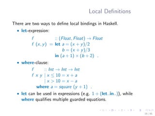
Local Definitions
There are two ways to define local bindings in Haskell.
• let-expression:
f :: (Float, Float) → Float
f (x, y) = let a = (x + y)/2
b = (x + y)/3
in (a + 1) × (b + 2) .
• where-clause:
f :: Int → Int → Int
f x y | x ≤ 10 = x + a
| x > 10 = x − a
where a = square (y + 1) .
• let can be used in expressions (e.g. 1 + (let..in..)), while
where qualifies multiple guarded equations.
19 / 85

Types
• The universe of values is partitioned into collections, called
types.
• Some basic types: Int, Float, Bool, Char. . .
• Type “constructors”: functions, lists, trees . . . to be
introduced later.
• Operations on values of a certain type might not make sense
for other types. For example: square square 3.
20 / 85

Strong Typing
• Strong typing: the type of a well-formed expression can be
deducted from the constituents of the expression.
• It helps you to detect errors.
• More importantly, programmers may consider the types for
the values being deﬁned before considering the deﬁnition
themselves, leading to clear and well-structured programs.
21 / 85

Booleans
The datatype Bool can be introduced with a datatype declaration:
data Bool = False | True .
(But you need not do so. The type Bool is already deﬁned in the
Haskell Prelude.)
22 / 85

Datatype Declaration
• In Haskell, a data declaration deﬁnes a new type.
data Type = Con1 Type11 Type12 . . .
| Con2 Type21 Type22 . . .
| :
• The declaration above introduces a new type, Type, with
several cases.
• Each case starts with a constructor, and several (zero or
more) arguments (also types).
• Informally it means “a value of type Type is either a Con1
with arguments Type11, Type12. . . , or a Con2 with arguments
Type21, Type22. . . ”
• Types and constructors begin in capital letters.
23 / 85

Functions on Booleans
Negation:
not :: Bool → Bool
not False = True
not True = False .
• Notice the definition by pattern matching. The definition has
two cases, because Bool is defined by two cases. The shape of
the function follows the shape of its argument.
24 / 85

Conjunction and disjunction:
(&&), (||) :: Bool → Bool → Bool
False && x = False
True && x = x ,
False || x = x
True || x = True .
25 / 85

Equality check:
(==), (=) :: Bool → Bool → Bool
x == y = (x && y) || (not x && not y)
x = y = not (x == y) .
• = is a deﬁnition, while == is a function.
• = is written / = in ASCII.
26 / 85

Example
leapyear :: Int → Bool
leapyear y = (y ‘mod‘ 4 == 0) &&
(y ‘mod‘ 100 = 0 || y ‘mod‘ 400 == 0) .
• Note: y ‘mod‘ 100 could be written mod y 100. The
backquotes turns an ordinary function to an inﬁx operator.
• It’s just personal preference whether to do so.
27 / 85

Characters
• You can think of Char as a big data deﬁnition:
data Char = 'a' | 'b' | . . .
with functions:
ord :: Char → Int
chr :: Int → Char .
• Characters are compared by their order:
isDigit :: Char → Bool
isDigit x = '0' ≤ x && x ≤ '9' .
28 / 85

Tuples
• The polymorphic type (a, b) is essentially the same as the
following declaration:
data Pair a b = MkPair a b .
• Or, had Haskell allow us to use symbols:
data (a, b) = (a, b) .
• Two projections:
fst :: (a, b) → a
fst (a, b) = a ,
snd :: (a, b) → b
snd (a, b) = b .
29 / 85

Either and Maybe
• Another standard datatype Either a b states that a value is
“either an a, or a b.”
data Either a b = Left a | Right b .
• Another standard datatype Either a b states that a value is
“either an a, or a b.”
data Maybe a = Just a | Nothing .
• We will see their usage in practicals.
30 / 85

Pattern Matching
• Previously, pattern matching only happens in the LHS of a
function deﬁnition:
f (x, y) = . . .
g (Left x) = . . .
g (Right x) = . . .
• You can also patten-match in a let-binding:
f x = let (y, z) = . . . in . . .
31 / 85

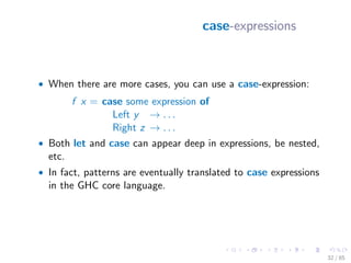
case-expressions
• When there are more cases, you can use a case-expression:
f x = case some expression of
Left y → . . .
Right z → . . .
• Both let and case can appear deep in expressions, be nested,
etc.
• In fact, patterns are eventually translated to case expressions
in the GHC core language.
32 / 85

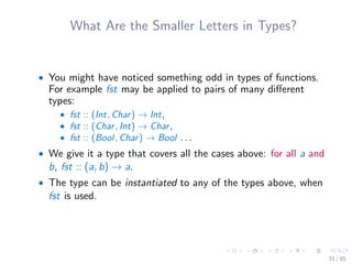
What Are the Smaller Letters in Types?
• You might have noticed something odd in types of functions.
For example fst may be applied to pairs of many diﬀerent
types:
• fst :: (Int, Char) → Int,
• fst :: (Char, Int) → Char,
• fst :: (Bool, Char) → Bool . . .
• We give it a type that covers all the cases above: for all a and
b, fst :: (a, b) → a.
• The type can be instantiated to any of the types above, when
fst is used.
33 / 85

Parametric Polymorphic Types
• Polymorphism: allowing one term to have many types.
• In the style we have seen above, the “many types” of fst are
selected by assigning diﬀerent types (Int, Bool, etc) to
parameters (a and b).
• This style is thus called parametric polymorphism.
• Note that, in this style, the same function (the same
algorithm) can be applied to many diﬀerent types, because it
does not matter to the algorithm what they are.
• E.g., fst does not need to know what a and b are in its input
(a, b).
34 / 85

Equality Check
• You might have also noticed that we can check for equality of
a number of types:
• (==) :: Char → Char → Bool,
• (==) :: Int → Int → Bool,
• (==) :: (Int, Char) → (Int, Char) → Bool,
• (==) :: [Int] → [Int] → Bool . . .
• It diﬀers from the situation of fst: the algorithm for checking
equality for each type is diﬀerent. We just use the same name
to refer to them, for convenience.
35 / 85

Equality Check
• Furthermore, not all types have (==) defined. For example,
we cannot check whether two functions are equal.
• (==) is an overloaded name — one name shared by many
different definitions of equalities, for different types.
• It is some times called ad-hoc polymorphism.
36 / 85

Ad-Hoc Polymorphism
• Haskell deals with overloading by a general mechanism called
type classes. It is considered a major feature of Haskell.
• While the type class is an interesting topic, we might not
cover much of it since it is orthogonal to the central message
of this course.
• We only need to know that if a function uses (==), it is
noted in the type.
• E.g. The function pos x xs finds the position of the first
occurrence of x in xs. It needs to use equality check.
• It my have type pos :: Eq a ⇒ a → [a] → Int.
• Eq a says that “a cannot be any type. It should be a type for
which (==) is defined.”
37 / 85

Lists in Haskell
• Lists: conceptually, sequences of things.
• Traditionally an important datatype in functional languages.
• In Haskell, all elements in a list must be of the same type.
• [1, 2, 3, 4] :: [Int]
• [True, False, True] :: [Bool]
• [[1, 2], [ ], [6, 7]] :: [[Int]]
• [ ] :: [a], the empty list (whose element type is not determined).
38 / 85

List as a Datatype
• [ ] :: [a] is the empty list whose element type is not determined.
• If a list is non-empty, the leftmost element is called its head
and the rest its tail.
• The constructor (:) :: a → [a] → [a] builds a list. E.g. in
x : xs, x is the head and xs the tail of the new list.
• You can think of a list as being deﬁned by
data [a] = [ ] | a : [a] .
• [1, 2, 3] is an abbreviation of 1 : (2 : (3 : [ ])).
39 / 85

Characters and Strings
• In Haskell, strings are treated as lists of characters.
• Thus when we write "abc", it is treated as an abbreviation of
['a', 'b', 'c'].
• It makes string processing convenient, while having some
eﬃciency issues.
• For eﬃciency, there are libraries providing “block”
representation of strings.
40 / 85

Head and Tail
• head :: [a] → a. e.g. head [1, 2, 3] = 1.
• tail :: [a] → [a]. e.g. tail [1, 2, 3] = [2, 3].
• init :: [a] → [a]. e.g. init [1, 2, 3] = [1, 2].
• last :: [a] → a. e.g. last [1, 2, 3] = 3.
• They are all partial functions on non-empty lists. e.g. head [ ]
crashes with an error message.
• null :: [a] → Bool checks whether a list is empty.
41 / 85

List Generation
• [0..25] generates the list [0, 1, 2..25].
• [0, 2..25] yields [0, 2, 4..24].
• [2..0] yields [].
• The same works for all ordered types. For example Char:
• ['a'..'z'] yields ['a', 'b', 'c'..'z'].
• [1..] yields the inﬁnite list [1, 2, 3..].
42 / 85

List Comprehension
• Some functional languages provide a convenient notation for
list generation. It can be deﬁned in terms of simpler functions.
• e.g. [x × x | x ← [1..5], odd x] = [1, 9, 25].
• Syntax: [e | Q1, Q2..]. Each Qi is either
• a generator x ← xs, where x is a (local) variable or pattern of
type a while xs is an expression yielding a list of type [a], or
• a guard, a boolean valued expression (e.g. odd x).
• e is an expression that can involve new local variables
introduced by the generators.
43 / 85

List Comprehension
Examples:
• [(a, b) | a ← [1..3], b ← [1..2]] =
[(1, 1), (1, 2), (2, 1), (2, 2), (3, 1), (3, 2)]
• [(a, b) | b ← [1..2], a ← [1..3]] =
[(1, 1), (2, 1), (3, 1), (1, 2), (2, 2), (3, 2)]
• [(i, j) | i ← [1..4], j ← [i + 1..4]] =
[(1, 2), (1, 3), (1, 4), (2, 3), (2, 4), (3, 4)]
• [(i, j) |← [1..4], even i, j ← [i + 1..4], odd j] = [(2, 3)]
44 / 85

Inductively Defined Lists
• Recall that a (finite) list can be seen as a datatype defined
by: 1
data [a] = [] | a : [a] .
• Every list is built from the base case [ ], with elements added
by (:) one by one: [1, 2, 3] = 1 : (2 : (3 : [ ])).
• The type [a] is the smallest set such that
1 [ ] is in [a];
2 if xs is in [a] and x is in a, x : xs is in [a] as well.
• In fact, Haskell allows you to build infinitely long lists (one
that never reaches [ ]). However. . .
• for now let’s consider finite lists only, as having infinite lists
make the semantics much more complicated. 2
1
Not a real Haskell definition.
2
What does that mean? We will talk about it later.
45 / 85

Inductively Defined Functions on Lists
• Many functions on lists can be defined according to how a list
is defined:
sum :: [Int] → Int
sum [ ] = 0
sum (x : xs) = x + sum xs .
allEven :: Int → Bool
allEven [ ] = True
allEven f (x : xs) = even x && allEven xs .
46 / 85

Length
• The function length deﬁned inductively:
length :: [a] → Int
length [ ] = 0
length (x : xs) = 1+ length xs .
47 / 85

List Append
• The function (++) appends two lists into one
(++) :: [a] → [a] → [a]
[ ] ++ ys = ys
(x : xs) ++ ys = x : (xs ++ ys) .
• Examples:
• [1, 2] ++[3, 4, 5] = [1, 2, 3, 4, 5],
• [ ] ++[3, 4, 5] = [3, 4, 5] = [3, 4, 5] ++[ ].
• Compare with (:) :: a → [a] → [a]. It is a type error to write
[ ] : [3, 4, 5]. (++) is deﬁned in terms of (:).
• Is the following true?
length (xs ++ ys) = length xs + length ys .
• In words, length distributes into (++).
• How can we convince ourselves that the property holds. That
is, how can we prove it?
48 / 85

Concatenation
• While (++) repeatedly applies (:), the function concat
repeatedly calls (++):
concat :: [[a]] → [a]
concat [ ] = [ ]
concat (xs : xss) = xs ++ concat xss .
• E.g. concat [[1, 2], [ ], [3, 4], [5]] = [1, 2, 3, 4, 5].
• Compare with sum.
• Is it always true that sum · concat = sum · map sum?
49 / 85

Definition by Induction/Recursion
• Rather than giving commands, in functional programming we
specify values; instead of performing repeated actions, we
define values on inductively defined structures.
• Thus induction (or in general, recursion) is the only “control
structure” we have. (We do identify and abstract over plenty
of patterns of recursion, though.)
• To inductively define a function f on lists, we specify a value
for the base case (f [ ]) and, assuming that f xs has been
computed, consider how to construct f (x : xs) out of f xs.
50 / 85

Filter
• filter :: (a → Bool) → [a] → [a].
• e.g. filter even [2, 7, 4, 3] = [2, 4]
• filter (λn → n ‘mod‘ 3 == 0) [3, 2, 6, 7] = [3, 6]
• Application: count the number of occurrences of a in a list:
• length · filter ('a' ==)
• Or length · filter (λx → 'a' == x)
51 / 85

Filter
• filter p xs keeps only those elements in xs that satisfy p.
filter :: (a → Bool) → [a] → [a]
filter p [ ] = [ ]
filter p (x : xs) | p x = x : filter p xs
| otherwise = filter p xs .
52 / 85

List Reversal
• reverse [1, 2, 3, 4] = [4, 3, 2, 1].
reverse :: [a] → [a]
reverse [ ] = [ ]
reverse (x : xs) = reverse xs ++[x] .
53 / 85

Map
• map :: (a → b) → [a] → [b] applies the given function to each
element of the input list, forming a new list.
• For example, map (1+) [1, 2, 3, 4, 5] = [2, 3, 4, 5, 6].
• map square [1, 2, 3, 4] = [1, 4, 9, 16].
• How do you deﬁne map inductively?
54 / 85

Map
• Observe that given f :: (a → b), map f is a function, of type
[a] → [b], that can be deﬁned inductively on lists.
map :: (a → b) → ([a] → [b])
map f [ ] = [ ]
map f (x : xs) = f x : map f xs .
55 / 85

Some More About Map
• Every once in a while you may need a small function which
you do not want to give a name to. At such moments you can
use the λ notation:
• map (λx → x × x) [1, 2, 3, 4] = [1, 4, 9, 16]
• Note: a list comprehension can always be translated into a
combination of primitive list generators and map, ﬁlter, and
concat.
56 / 85

TakeWhile
• takeWhile p xs yields the longest preﬁx of xs such that p
holds for each element.
• E.g. takeWhile even [2, 4, 5, 6, 8] = [2, 4].
57 / 85

TakeWhile
• takeWhile p xs yields the longest preﬁx of xs such that p
holds for each element.
• E.g. takeWhile even [2, 4, 5, 6, 8] = [2, 4].
• Inductive deﬁnition:
takeWhile :: (a → Bool) → [a] → [a]
takeWhile p [ ] = [ ]
takeWhile p (x : xs)
| p x = x : takeWhile p xs
| otherwise = [ ] .
57 / 85

DropWhile
• dropWhile p xs drops the preﬁx from xs.
• E.g. dropWhile even [2, 4, 5, 6, 8] = [5, 6, 8].
• Property: takeWhile p xs ++ dropWhile p xs = xs.
58 / 85

DropWhile
• dropWhile p xs drops the preﬁx from xs.
• E.g. dropWhile even [2, 4, 5, 6, 8] = [5, 6, 8].
• Inductive deﬁnition:
dropWhile :: (a → Bool) → [a] → [a]
dropWhile p [ ] = [ ]
dropWhile p (x : xs)
| p x = dropWhile p xs
| otherwise = x : xs .
• Property: takeWhile p xs ++ dropWhile p xs = xs.
58 / 85

All Preﬁxes and Suﬃxes
• inits [1, 2, 3] = [[ ], [1], [1, 2], [1, 2, 3]]
inits :: [a] → [[a]]
inits [ ] = [[ ]]
inits (x : xs) = [ ] : map (x :) (inits xs) .
• tails [1, 2, 3] = [[1, 2, 3], [2, 3], [3], [ ]]
tails :: [a] → [[a]]
tails [ ] = [[ ]]
tails (x : xs) = (x : xs) : tails xs .
59 / 85

Totality
• Structure of our deﬁnitions so far:
f [ ] = . . .
f (x : xs) = . . . f xs . . .
• Both the empty and the non-empty cases are covered,
guaranteeing there is a matching clause for all inputs.
• The recursive call is made on a “smaller” argument,
guranteeing termination.
• Together they guarantee that every input is mapped to some
output. Thus they deﬁne total functions on lists.
60 / 85

The So-Called “Mathematical Induction”
• Let P be a predicate on natural numbers.
• We’ve all learnt this principle of proof by induction: to prove
that P holds for all natural numbers, it is suﬃcient to show
that
• P 0 holds;
• P (1 + n) holds provided that P n does.
61 / 85

Proof by Induction on Natural Numbers
• We can see the above inductive principle as a result of seeing
natural numbers as defined by the datatype 3
data N = 0 | 1+ N .
• That is, any natural number is either 0, or 1+ n where n is a
natural number.
• The type N is the smallest set such that
1 0 is in N;
2 if n is in N, so is 1+ n.
• Thus to show that P holds for all natural numbers, we only
need to consider these two cases.
• In this lecture, 1+ is written in bold font to emphasise that it
is a data constructor (as opposed to the function (+), to be
defined later, applied to a number 1).
3
Not a real Haskell definition.
62 / 85

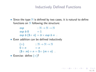
Inductively Defined Functions
• Since the type N is defined by two cases, it is natural to define
functions on N following the structure:
exp :: N → N → N
exp b 0 = 1
exp b (1+ n) = b × exp b n .
• Even addition can be defined inductively
(+) :: N → N → N
0 + n = n
(1+ m) + n = 1+ (m + n) .
• Exercise: define (×)?
63 / 85

Without the n + k Pattern
• Unfortunately, newer versions of Haskell abandoned the
“n + k pattern” used in the previous slide. And there is not a
built-in type for N. Instead we have to write:
exp :: Int → Int → Int
exp b 0 = 1
exp b n = b × exp b (n − 1) .
• For the purpose of this course, the pattern 1 + n reveals the
correspondence between N and lists, and matches our proof
style. Thus we will use it in the lecture.
• Remember to remove them in your code.
64 / 85

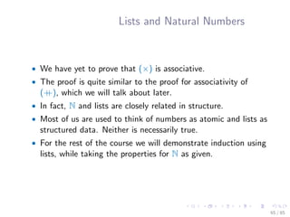
Lists and Natural Numbers
• We have yet to prove that (×) is associative.
• The proof is quite similar to the proof for associativity of
(++), which we will talk about later.
• In fact, N and lists are closely related in structure.
• Most of us are used to think of numbers as atomic and lists as
structured data. Neither is necessarily true.
• For the rest of the course we will demonstrate induction using
lists, while taking the properties for N as given.
65 / 85

Take and Drop
• take n takes the ﬁrst n elements of the list.
• For example, take 0 xs = [],
• take 3 "abcde" = "abc",
• take 3 "ab" = "ab".
• Dually, drop n drops the ﬁrst n elements of the list.
• For example, drop 0 xs = xs,
• drop 3 "abcde" = "cd",
• drop 3 "ab" = "".
• take n xs ++ drop n xs = xs, as long as evaluation of n
terminates.
66 / 85

Take and Drop
• They can be deﬁned by induction on the ﬁrst argument:
take :: N → [a] → [a]
take 0 xs = [ ]
take (1+ n) [ ] = [ ]
take (1+ n) (x : xs) = x : take n xs .
•
drop :: N → [a] → [a]
drop 0 xs = xs
drop (1+ n) [ ] = [ ]
drop (1+ n) (x : xs) = drop n xs .
• Note: take n xs ++ drop n xs = xs, for all n and xs.
67 / 85

Variations with the Base Case
• Some functions discriminate between several base cases. E.g.
fib :: N → N
fib 0 = 0
fib 1 = 1
fib (2 + n) = fib (1 + n) + fib n .
68 / 85

• Some functions make more sense when it is defined only on
non-empty lists:
f [x] = . . .
f (x : xs) = . . .
• What about totality?
• They are in fact functions defined on a different datatype:
data [a]+
= Singleton a | a : [a]+
.
• We do not want to define map, filter again for [a]+
. Thus we
reuse [a] and pretend that we were talking about [a]+
.
• It’s the same with N. We embedded N into Int.
• Ideally we’d like to have some form of subtyping. But that
makes the type system more complex.
69 / 85

Lexicographic Induction
• It also occurs often that we perform lexicographic induction
on multiple arguments: some arguments decrease in size,
while others stay the same.
• E.g. the function merge merges two sorted lists into one
sorted list:
merge :: [Int] → [Int] → [Int]
merge [ ] [ ] = [ ]
merge [ ] (y : ys) = y : ys
merge (x : xs) [ ] = x : xs
merge (x : xs) (y : ys)
| x ≤ y = x : merge xs (y : ys)
| otherwise = y : merge (x : xs) ys .
70 / 85

Zip
• zip :: [a] → [b] → [(a, b)]
• e.g. zip "abcde" [1, 2, 3] = [('a', 1), ('b', 2), ('c', 3)]
• The length of the resulting list is the length of the shorter
input list.
71 / 85

Zip
zip :: [a] → [b] → [(a, b)]
zip [ ] [ ] = [ ]
zip [ ] (y : ys) = [ ]
zip (x : xs) [ ] = [ ]
zip (x : xs) (y : ys) = (x, y) : zip xs ys .
72 / 85

Non-Structural Induction
• In most of the programs we’ve seen so far, the recursive call
are made on direct sub-components of the input (e.g.
f (x : xs) = ..f xs..). This is called structural induction.
• It is relatively easy for compilers to recognise structural
induction and determine that a program terminates.
• In fact, we can be sure that a program terminates if the
arguments get “smaller” under some (well-founded) ordering.
73 / 85

Mergesort
• In the implemenation of mergesort below, for example, the
arguments always get smaller in size.
msort :: [Int] → [Int]
msort [ ] = [ ]
msort [x] = [x]
msort xs = merge (msort ys) (msort zs) ,
where n = length xs ‘div‘ 2
ys = take n xs
zs = drop n xs .
• What if we omit the case for [x]?
• If all cases are covered, and all recursive calls are applied to
smaller arguments, the program deﬁnes a total function.
74 / 85

A Non-Terminating Deﬁnition
• Example of a function, where the argument to the recursive
does not reduce in size:
f :: Int → Int
f 0 = 0
f n = f n .
• Certainly f is not a total function. Do such deﬁnitions
“mean” something? We will talk about these later.
75 / 85

A Common Pattern We’ve Seen Many
Times. . .
• Many programs we have seen follow a similar pattern:
sum [ ] = 0
sum (x : xs) = x + sum xs .
length [ ] = 0
length (x : xs) = 1 + length xs .
map f [ ] = [ ]
map f (x : xs) = f x : map f xs .
• This pattern is extracted and called foldr:
foldr f e [ ] = e
foldr f e (x : xs) = f x (foldr f e xs) .
76 / 85

Replacing Constructors
• The function foldr is among the most important functions on
lists.
foldr :: (a → b → b) → b → [a] → b
• One way to look at foldr (⊕) e is that it replaces [ ] with e
and (:) with (⊕):
foldr (⊕) e [1, 2, 3, 4]
= foldr (⊕) e (1 : (2 : (3 : (4 : [ ]))))
= 1 ⊕ (2 ⊕ (3 ⊕ (4 ⊕ e))).
• sum = foldr (+) 0.
• One can see that id = foldr (:) [ ].
77 / 85

Some Trivial Folds on Lists
• Function maximum returns the maximum element in a list:
• Function prod returns the product of a list:
• Function and returns the conjunction of a list:
• Lets emphasise again that id on lists is a fold:
78 / 85

• maximum = foldr max -∞.
78 / 85

• prod = foldr (×) 1.
78 / 85

• and = foldr (&&) True.
78 / 85

• and = foldr (&&) True.
• id = foldr (:) [ ].
78 / 85

Some Slightly Complex Folds
• length = foldr (λx n → 1 + n) 0.
• map f = foldr (λx xs → f x : xs) [ ].
• xs ++ ys = foldr (:) ys xs. Compare this with id!
• filter p = foldr (fil p) [ ]
where fil p x xs = if p x then (x : xs) else xs.
79 / 85

The Ubiquitous Fold
• In fact, any function that takes a list as its input can be
written in terms of foldr — although it might not be always
practical.
• With fold it comes one of the most important theorem in
program calculation — the fold-fusion theorem. We will talk
about it later.
80 / 85

Internally Labelled Binary Trees
• This is a possible deﬁnition of internally labelled binary trees:
data Tree a = Null | Node a (Tree a) (Tree a) ,
• on which we may inductively deﬁne functions:
sumT :: Tree N → N
sumT Null = 0
sumT (Node x t u) = x + sumT t + sumT u .
81 / 85

Exercise: given (↓) :: N → N → N, which yields the smaller one of
its arguments, deﬁne the following functions
1 minT :: Tree N → N, which computes the minimal element in
a tree.
2 mapT :: (a → b) → Tree a → Tree b, which applies the
functional argument to each element in a tree.
3 Can you deﬁne (↓) inductively on N? 4
4
In the standard Haskell library, (↓) is called min.
82 / 85

• Every inductively deﬁned datatype comes with its induction
principle.
• We will come back to this point later.
83 / 85

Recommanded Textbooks
• Introduction to Functional Programming using Haskell. My
recommended book. Covers equational reasoning very well.
• Programming in Haskell. A thin but complete textbook.
84 / 85

Online Haskell Tutorials
• Learn You a Haskell for Great Good! , a nice tutorial with
cute drawings!
• Yet Another Haskell Tutorial.
• A Gentle Introduction to Haskell by Paul Hudak, John
Peterson, and Joseph H. Fasel: a bit old, but still worth a
read.
• Real World Haskell. Freely available online. It assumes some
basic knowledge of Haskell, however.
85 / 85

[FLOLAC'14][scm] Functional Programming Using Haskell

More Related Content

What's hot (15)

Viewers also liked (20)

Similar to [FLOLAC'14][scm] Functional Programming Using Haskell (20)

Recently uploaded (20)

[FLOLAC'14][scm] Functional Programming Using Haskell