Gradient_Descent_Unconstrained.pdf

Fall 2022
Gradient Descent Method
Course: SDS 384
Instructor: Nhat Ho
1

• Apart from foundational aspects of gradient descent method, our lecture will
also involve:
• Concentration inequalities with a sequence of random variables (You
can read more about this topic from Section 2 to Section 5 in [1])
• Research questions that you can use for your final project or your
research topic
• We will focus on the trade-oﬀ between statistical complexity and
computational eﬃciency of gradient descent method in machine learning
models
• It yields useful insight into the practice of gradient descent method
• It leads to a design of optimal optimization algorithms for certain
machine learning models
2

Gradient Descent: Motivation
• Gradient descent is perhaps the simplest optimization algorithm
• It is simple to implement and has low computational complexity, which fits to large-scale
machine learning problems
• Asymptotic behaviors of gradient descent had been understood quite well
• Research problems: Understanding the non-asymptotic behaviors of gradient descent and
its variants has still remained an active important research area
• How many data samples are needed for gradient descent to reach a certain
neighborhood around the true value?
• For adaptive gradient methods, like Adam/ Adagrad/ Polyak average step size, the
trade-oﬀ between their statistical guarantee and their computational complexity
remained poorly understood
• How to develop uncertainty quantification for (adaptive) gradient descent iterates,
such as confidence intervals, etc.?
3

Example: Generalized Linear Model
• Assume that we have a generalized linear model:
,
where are response variables;
are covariates;
are i.i.d. (independently identical distributed) random noises
from ;
: a given link function (e.g, —linear regression model;
— phase retrieval problem)
Goal: Estimate true but unknown parameter
Yi = g(X⊤
i θ*) + εi, for i = 1,…, n
Y1, …, Yn ∈ ℝ
X1, …, Xn ∈ ℝd
ε1, …, εn
𝒩(0,1)
g g(x) = x
g(x) = x2
θ* ∈ ℝd
Sample size
4

• Least-square loss:
• In general, for non-linear link function , such as for , we do
not have closed-form expression for the optimal solution
• We use gradient descent algorithm to approximate the optimal solution
• Denote : iterate of gradient descent at step ,
: optimal solution of the least-square loss
min
θ∈ℝd
ℒn(θ) =
1
n
n
∑
i=1
{Yi − g(X⊤
i θ)}2
g g(x) = xp
p > 1
θt
n t
̂
θn
5

θ0
n
θ1
n
θ2
n
…..
θ*
̂
θn θt
n
r*
n
rt
n
: Radius of convergence
r*
n
: Current radius from step t
rt
n
Research Questions: (Q.1) For a fixed , can we develop (tight) bounds for ?
(Q.2) What is the lower bound for such that
for some universal constant
(Q.3) What is a good confidence interval for for fixed ?
t rt
n
t rt
n ≤ Cr*
n
C
θt
n t
6

• These open questions require the following deep understandings:
• Model perspective: The optimization landscape of generalized linear
model or machine learning models in general
• Optimization perspective: The dynamics of gradient descent algorithm
and its variants
• Statistical perspective: The concentration behaviors of the least-square
loss and its derivatives, i.e., for fixed sample size, how close the least-
square loss and its derivatives to their expectations?
• We will first focus on the optimization perspective of gradient descent method
7

Unconstrained Optimization:
Global Strong Convexity and Smoothness
8

Unconstrained Optimization
• We first consider general unconstrained optimization problems
• Assume that is an objective function that is diﬀerentiable
• The unconstrained optimization problem is given by:
• We use gradient descent method to approximate the optimal solution of
that problem
f : ℝd
→ ℝ
min
θ∈ℝd
f(θ)
θ*
9

• Assume that we start with an initialization
• We would like to build an iterative scheme such that
for any
• Gradient descent method:
,
where step size/ learning rate (may also be adaptive with )
θ0
θt+1
= F(θt
)
f(θt+1
) < f(θt
)
t ≥ 0
θt+1
= θt
− ηt ∇f(θt
)
ηt > 0 : t
10

θ0
θ1
θ2
θ3
Illustration of gradient descent method
• Gradient descent finds steepest descent
at the current iteration
• Descent direction at :
• Simple application of Cauchy-Schwarz:
where the equality holds when
θt
d θt
d⊤
∇f(θt
) < 0
min
∥d∥≤1
d⊤
∇f(θt
) = −∥∇f(θt
)∥
d = −
∇f(θt
)
∥∇f(θt)∥
11

Strong Convexity
• If is second order diﬀerentiable, i.e., second order derivative exists, strong
convexity is equivalent to
,
for all where smallest eigenvalue of matrix
• We call to be -strongly convex function
• That notion also implies that
,
for all
f
λmin(∇2
f(θ)) ≥ μ > 0
θ λmin(A) : A
f μ
f(θ) ≥ f(θ′) + ⟨∇f(θ′), θ − θ′⟩ +
μ
2
∥θ − θ′∥2
θ, θ′ ∈ ℝd
12

Strongly Convexity
• Examples of strongly convex function:
• Indeed, we have , which has smallest eigenvalue to be 2
• Therefore, function is 2-strongly convex
• Note that, when for and , the function is no
longer strongly convex (Check that!)
f(θ) = ∥θ∥2
∇2
f(θ) = 2 ⋅ Id
f
f(θ) = ∥θ∥2p
p ∈ ℕ p ≥ 2 f
This kind of behavior appears in several machine learning models, such
as generalized linear models, mixture models, matrix completion/ sensing,
deep neural networks, etc. 13

Smoothness
• The function is -smooth if is second order diﬀerentiable and
,
for all where largest eigenvalue of matrix
• That notion also implies that
,
for all
• If , then
•
• The function is 2-smooth
f L f
λmax(∇2
f(θ)) ≤ L
θ λmax(A) : A
f(θ) ≤ f(θ′) + ⟨∇f(θ′), θ − θ′⟩ +
L
2
∥θ − θ′∥2
θ, θ′ ∈ ℝd
f(θ) = ∥θ∥2
λmax(∇2
f(θ)) = 2
f
14

Convergence Rate: Strong Convexity and Smoothness
Theorem 1: Assume that the function is -strongly convex and -smooth. As long as
, we obtain that
f μ L
ηt = η ≤
1
L
∥θt
− θ*∥ ≤ (1 − η ⋅ μ)
t
2
∥θ0
− θ*∥
• It shows that converges geometrically fast to
•
When , the contraction coeﬃcient becomes ,
where is a condition number
• We can improve the upper bound of to (Not the focus of the class)
θt
θ*
η =
1
L
1 −
μ
L
= 1 −
1
κ
κ
η
2
L + μ
15

Lemma 1: If is -strongly convex and -smooth function, then
f μ L
2μ(f(θ) − f(θ*)) ≤ ∥∇f(θ)∥2
≤ 2L(f(θ) − f(θ*))
Proof of Lemma 1: From the strong convexity, we have
• Similar argument for the upper bound
f(θ) − f(θ*) ≤ ⟨∇f(θ), θ − θ*⟩ −
μ
2
∥θ − θ*∥2
= −
1
2
∥ μ(θ − θ*) −
1
μ
∇f(θ)∥2
+
1
2μ
∥∇f(θ)∥2
≤
1
2μ
∥∇f(θ)∥2
16

Convergence Rate: Strong convexity and Smoothness
Proof of Theorem 1:
•
(1)
• Strong convexity indicates
(2)
• Equations (1) and (2) lead to
(3)
∥θt+1
− θ*∥2
= ∥θt
− θ* − η∇f(θt
)∥2
= ∥θt
− θ*∥2
− 2η⟨∇f(θt
), θt
− θ*⟩ + η2
∥∇f(θt
)∥2
μ−
f(θ*) ≥ f(θt
) + ⟨∇f(θt
), θ* − θt
⟩ +
μ
2
∥θt
− θ*∥2
∥θt+1
− θ*∥2
≤ (1 − η ⋅ μ)∥θt
− θ*∥2
+ 2η(f(θ*) − f(θt
)) + η2
∥∇f(θt
)∥2
17

Convergence Rate: Strong convexity and Smoothness
• Use Lemma 1 to equation (3):
• As , we have
• Therefore, we find that:
• Repeat this argument, we obtain the conclusion of Theorem 1
∥θt+1
− θ*∥2
≤ (1 − η ⋅ μ)∥θt
− θ*∥2
+ (2Lη2
− 2η)(f(θt
) − f(θ*))
η ≤
1
L
2Lη2
≤ 2η
∥θt+1
− θ*∥2
≤ (1 − η ⋅ μ)∥θt
− θ*∥2
18

Corollary 1: Assume that the function is -strongly convex and -smooth. As
long as , we obtain that
f μ L
ηt = η ≤
1
L
f(θt
) − f(θ*) ≤
L
2
(1 − η ⋅ μ)
t
∥θ0
− θ*∥2
19

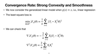
• We now consider the generalized linear model when , i.e., linear regression
• The least-square loss is:
• We can check that
;
g(x) = x
min
θ∈ℝd
ℒn(θ) =
1
n
n
∑
i=1
{Yi − X⊤
i θ}2
∇ℒn(θ) = −
2
n
n
∑
i=1
Xi(Yi − X⊤
i θ)
∇2
ℒn(θ) =
2
n
n
∑
i=1
XiX⊤
i
20

• To simplify the understanding, consider one dimensional problem, i.e,
• Assume that
•
• From the concentration inequality of chi-square distribution (see Example 2.11 in [1]),
,
where the outer expectation is taken with respect to
d = 1
Xi ∼ 𝒩(0,1)
∇2
ℒn(θ) =
2
n
n
∑
i=1
X2
i
ℙ
1
n
n
∑
i=1
X2
i − 𝔼(X2
) ≥ t ≤ 2 exp(−n ⋅ t2
/8)
X ∼ 𝒩(0,1)
21

• We have as
• It suggests that with probability for some ,
,
where is some universal constant
•
As , it demonstrates that with probability :
: =
The function is -smooth and -strongly convex
𝔼(X2
) = 1 X ∼ 𝒩(0,1)
1 − δ δ > 0
1
n
n
∑
i=1
X2
i − 1 ≤
C ⋅ log(1/δ)
n
C
∇2
ℒn(θ) =
2
n
n
∑
i=1
X2
i 1 − δ
μ =: 2 −
C ⋅ log(1/δ)
n
≤ ∇2
ℒn(θ) ≤ 2 +
C ⋅ log(1/δ)
n
L
ℒn L μ 22

•
Recall the least-square loss
• Denote by the optimal solution of least-square loss
• From Theorem 1, if we call the gradient descent iterate at step , then with
high probability
as long as
min
θ∈ℝd
1
n
n
∑
i=1
(Yi − Xi ⋅ θ)2
̂
θn
θt
n t
∥θt
n − ̂
θn∥ ≤ (1 − η ⋅ μ)t/2
∥θ0
n − ̂
θn∥
η ≤
1
L
23

• Recall that, we would like to estimate , a true but unknown parameter, of
the true model:
• (Q.1): For a fixed , what is an upper bounds for ?
• Our result with gradient descent sequence shows that
(Triangle inequality)
(4)
• It answers question (Q.1) earlier in first slides
θ*
Yi = Xi ⋅ θ* + εi
t ∥θt
n − θ*∥
{θt
n}t≥0
∥θt
n − θ*∥ ≤ ∥θt
n − ̂
θn∥ + ∥ ̂
θn − θ*∥
≤ (1 − η ⋅ μ)t/2
∥θ0
n − ̂
θn∥ + ∥ ̂
θn − θ*∥
Optimization error Statistical error
24

• (Q.2): The number of iterations such that reaches the radius of
convergence:
t θt
n
∥θt
n − θ*∥ ≤ C′∥ ̂
θn − θ*∥
θ*
̂
θn θt
n
r*
n
rt
n
25

• Recall from equation (4) that:
• We choose such that , i.e.,
,
where is such that
• Therefore, we need for some constant to answer question (Q.2)
∥θt
n − θ*∥ ≤ (1 − η ⋅ μ)t/2
∥θ0
n − ̂
θn∥ + ∥ ̂
θn − θ*∥
t (1 − η ⋅ μ)t/2
∥θ0
n − ̂
θn∥ ≤ ∥ ̂
θn − θ*∥
t ≤
2 log (∥ ̂
θn − θ*∥/C)
log(1 − η ⋅ μ)
≈ log(n)
C ∥θ0
n − ̂
θn∥ ≤ C
t ≥ c ⋅ log n c
26

• Takeaway messages: Under the strongly convex and smooth settings of the
loss function, we can have a good understanding of:
• The range of gradient descent updates at fixed number of iterates
• The suﬃcient number of iterations for the gradient descent
updates to reach the radius of convergence
• Remaining problems:
• When the loss function is not strongly convex or smooth, analyzing the
updates of gradient descent becomes more challenging
27

Local Strong Convexity and Local
Smoothness
28

Local Smoothness
• We now consider the generalized linear model when , i.e., quadratic
regression or phase retrieval problem
• The phase retrieval least-square loss function in one dimension is:
• We first assume that (The case will be considered later)
• We will show that the loss function is not strongly convex (It is indeed non-
convex problem)
g(x) = x2
min
θ∈ℝ
ℒn(θ) =
1
n
n
∑
i=1
{Yi − (Xi ⋅ θ)2
}2
=
(
1
n
n
∑
i=1
X4
i
)
θ4
−
(
2
n
YiX2
i )
θ2
+
1
n
n
∑
i=1
Y2
i
θ* ≠ 0 θ* = 0
ℒn
29

Local Smoothness
• Direct calculation shows that
,
• Recall that, where and
• By solving = 0, we obtain with high probability that is local maxima and
are two global minima
∇ℒn(θ) =
(
4
n
n
∑
i=1
X4
i
)
θ3
−
4
n
(
n
∑
i=1
YiX2
i )θ
∇2
ℒn(θ) =
(
12
n
n
∑
i=1
X4
i
)
θ2
−
4
n
(
n
∑
i=1
YiX2
i )
Yi = (Xi ⋅ θ*)2
+ εi Xi ∼ 𝒩(0,1) θ* ≠ 0
∇ℒn(θ) θ = 0
θ = ±
∑
n
i=1
YiX2
i
∑
n
i=1
X4
i
30

Local Smoothness
•
Both and are bounded with high probability (We
ignore the rigorousness here)
• It demonstrates that when , with high probability
• Hence, the loss function is not globally smooth (Recall that, we need
step size . Therefore, as , the upper bound for step size goes
to 0, which is bad!)
12
n
n
∑
i=1
X4
i 4(
n
∑
i=1
YiX2
i )
θ → ∞ ∇2
ℒn(θ) → ∞
ℒn
η ≤ 1/L L → ∞
31

Local Smoothness
•
• If we indeed consider , then we
can find depending on such that with high probability
,
for all where is an optimal solution of
• It demonstrates that the function is locally smooth around
∇2
ℒn(θ) =
(
12
n
n
∑
i=1
X4
i
)
θ2
− 4(
n
∑
i=1
YiX2
i )
θ ∈ 𝔹( ̂
θn, r0) = {θ′ ∈ ℝ : ∥θ′− ̂
θn∥ ≤ r0}
L1 r0
∇2
ℒn(θ) ≤ L1
θ ∈ 𝔹( ̂
θn, r0) ̂
θn ℒn
̂
θn
32

Local Strong Convexity
•
Recall that,
•
We know that
•
The Hessian is zero when
• It shows that we not always have bounded away from 0 when
where (here we assume , have the same sign)
∇2
ℒn(θ) =
(
12
n
n
∑
i=1
X4
i
)
θ2
−
4
n
(
n
∑
i=1
YiX2
i )
̂
θn = ±
∑
n
i=1
YiX2
i
∑
n
i=1
X4
i
θ̄n = ±
∑
n
i=1
YiX2
i
3∑
n
i=1
X4
i
∇2
ℒn(θ)
θ ∈ 𝔹( ̂
θn, r) r ≥ ∥θ̄n − ̂
θn∥ θ̄n
̂
θn
33

• This example shows that as long as for some small
, the function is locally strongly convex around
• Combining with the local smoothness argument earlier, the ball
is suﬃcient to guarantee that the function is locally
strongly convex and smooth around
r = ∥θ̄n − ̂
θn∥ − ϵ
ϵ > 0 ℒn
̂
θn
𝔹( ̂
θn,∥ ̂
θn − θ̄n∥ − ϵ) ℒn
̂
θn
34

• We now consider another popular example of local strong convexity: logistic
regression
• For logistic regression, we assume that and
where is unknown true parameter
• We estimate the true parameter via maximum likelihood estimation
Yi ∈ {−1,1}
ℙ(Yi = 1|Xi) =
exp(X⊤
i θ*)
1 + exp(X⊤
i θ*)
θ*
θ*
35

• It is equivalent to:
• Some algebra shows that
• When ,
• The function is not globally strongly convex (In fact, it is locally strongly
convex around the global maxima)
max
θ∈ℝd
𝒯n(θ) =
1
n
n
∑
i=1
log(1 + exp(−YiX⊤
i θ))
∇2
𝒯n(θ) =
1
n
n
∑
i=1
exp(−YiX⊤
i θ)
(1 + exp(−YiX⊤
i θ))2
XiX⊤
i
∥θ∥ → ∞ λmin(∇2
𝒯n(θ)) → 0
𝒯n
36

Local Strong Convexity and Smoothness
• We now generalize the previous setting of phase retrieval into a general local
strong convexity setting:
,
where is locally -strongly convex and -smooth in the ball , i.e.,
,
for all
• Note that, for local strong convexity, it also happens to many machine learning
models, such as logistic regression
min
θ∈ℝd
f(θ)
f μ L 𝔹(θ*, r)
μ ≤ λmin(∇2
f(θ)) ≤ λmax(∇2
f(θ)) ≤ L
θ ∈ 𝔹(θ*, r)
37

Convergence rate: Local Strong Convexity and Smoothness
Theorem 2: Assume that the function is locally -strongly convex and -smooth in
where , is an initialization, and is the minimizer of . As
long as , we obtain that
f μ L
𝔹(θ*, r) r = ∥θ0
− θ*∥ θ0
θ* f
ηt = η ≤
1
L
∥θt
− θ*∥ ≤ (1 − η ⋅ μ)
t
2
∥θ0
− θ*∥
Proof sketch: Use idea of the proof of Theorem 1, we can prove that
as long as .
• It suggests that and we obtain the conclusion of the theorem
∥θt+1
− θ*∥2
≤ (1 − η ⋅ μ)∥θt
− θ*∥2
θt
∈ 𝔹(θ*, r)
θt+1
∈ 𝔹(θ*, r)
38

Example: Local Strong Convexity and Smoothness
• We now recall the phase retrieval problem earlier where the loss function
is locally strongly convex
• Assume that is the local initialization of and where is
some given small radius and is an optimal solution of
• There exist some constants and such that is locally -strongly
convex and -smooth in
• Denote by the sequence of gradient descent updates for solving the
loss
ℒn
θ0
n ℒn θ0
n ∈ 𝔹( ̂
θn, r0) r0
̂
θn ℒn
μ1 L1 ℒn μ1
L1 𝔹( ̂
θn, r0)
{θt
n}t≥0
ℒn
39

Example: Local Strong Convexity and Smoothness
• From Theorem 2:
• Therefore, we also obtain
• Furthermore, we also can derive other results of phase retrieval problem as
the strong convexity setting of linear regression problem
∥θt
n − ̂
θn∥ ≤ (1 − η ⋅ μ1)t/2
∥θ0
n − ̂
θn∥
∥θt
n − θ*∥ ≤ (1 − η ⋅ μ1)t/2
∥θ0
n − ̂
θn∥ + ∥ ̂
θn − θ*∥
40

Polyak-Lojasiewicz (PL) Condition
41

Beyond local convergence: Polyak-Lojasiewicz (PL) Condition
• An issue with local convergence is the local initialization
• We would like to have some guarantee beyond local convergence even when
the loss function is not globally strongly convex and smooth
• An important notion is Polyak-Lojasiewicz (PL) condition
Definition 1 (PL condition): Assume that is the loss function. The PL condition
entails that there exists such that
,
for all where is the minimizer of
f
μ > 0
∥∇f(θ)∥2
≥ 2μ(f(θ) − f(θ*))
θ ∈ ℝd
θ* f
42

• If the function is strongly convex, it satisfies the PL condition
• The PL condition guarantees that:
• All stationary points are global minimizers (not need to be unique)
• It mimics the condition on the lower bound of the smallest
eigenvalue of the Hessian matrix
• This condition also motivates the Polyak average step size adaptive
gradient descent (We will study it later)
PL
Strong Convexity
43

• Theorem 2 guarantees global linear convergence of the objective value from
any initialization θ0
Theorem 3: Assume that the function satisfies the PL condition for some .
Furthermore, is -smooth. As long as , we obtain that
f μ > 0
f L ηt = η =
1
L
| f(θt
) − f(θ*)| ≤
(
1 −
μ
L )
t
| f(θ0
) − f(θ*)|
44

• Proof of Theorem 2: Since is -smooth, we have
(5)
f L
f(θt
) ≤ f(θt−1
) + ⟨∇f(θt−1
), θt
− θt−1
⟩ +
L
2
∥θt
− θt−1
∥2
= f(θt−1
) − η∥∇f(θt−1
)∥2
+
η2
L
2
∥∇f(θt−1
)∥2
= f(θt−1
) −
1
2L
∥∇f(θt−1
)∥2
45

• An application of equation (5) and PL condition leads to
• Repeating the above argument, we obtain the conclusion
f(θt
) − f(θ*) ≤ f(θt−1
) − f(θ*) −
1
2L
∥∇f(θt−1
)∥2
≤ f(θt−1
) − f(θ*) −
μ
L
(f(θt−1
) − f(θ*))
=
(
1 −
μ
L)
(f(θt−1
) − f(θ*))
46

Example: Polyak-Lojasiewicz (PL) Condition
• We consider the high dimensional regression problem, i.e., generalized linear model
when and (the number of features is more than the number of
samples)
• The least-square loss is:
• , which is low rank since , where
• It means that
g(x) = x n < d
min
θ∈ℝd
ℒn(θ) =
1
n
n
∑
i=1
{Yi − X⊤
i θ}2
∇2
ℒn(θ) =
2
n
X⊤
X ∈ ℝd×d
n < d
X =
X1
X2
…
Xn
∈ ℝn×d
λmin(∇2
ℒn(θ)) = 0 47

• We will demonstrate that satisfies the PL condition
• In fact, if we call as the optimal solution of , we have (due to the
over-parametrized condition)
•
Direct calculation shows where
• Hence,
ℒn
̂
θn ℒn ℒn( ̂
θn) = 0
∇ℒn(θ) =
2
n
X⊤
(Xθ − Y) Y =
Y1
Y2
…
Yn
∈ ℝn
∥∇ℒn(θ)∥2
=
4
n2
(Xθ − Y)⊤
XX⊤
(Xθ − Y)
≥
4
n2
λmin(XX⊤
)∥Xθ − Y∥2
=
4λmin(XX⊤
)
n
(ℒn(θ) − ℒn( ̂
θn))
48

• It indicates that the loss function satisfies PL condition with constant
• Furthermore, is -smooth
• An application of Theorem 3 leads to
,
where is a sequence of gradient descent iterates
ℒn
4λmin(XX⊤
)
n
ℒn
2λmax(X⊤
X)
n
|ℒn(θt
n) − ℒn( ̂
θn)| ≤
(
1 −
2λmin(XX⊤
)
λmax(X⊤X) )
t
|ℒn(θ0
n) − ℒn( ̂
θn)|
{θt
n}t≥0
49

• Since there are multiple global minimum of the least-square loss, it implies that
• The updates from gradient descent converge to the closest minimum of
the initialization
• The PL condition is uniform, i.e., ,
for all
• This condition can be strong for several complex machine learning models,
such as reinforcement learning models
• We can adapt the PL condition to hold non-uniformly:
, for all where is some function
of and develop normalized version of gradient descent to account for the
non-uniformity (See paper [2] for detailed development)
∥∇f(θ)∥2
≥ 2μ(f(θ) − f(θ*))
θ ∈ ℝd
∥∇f(θ)∥2
≥ 2μ(θ)(f(θ) − f(θ*)) θ ∈ ℝd
μ(θ)
θ
50

Beyond Linear Convergence: Convex
Settings
51

Beyond Linear Convergence
• Thus far, we have the linear convergence of the gradient descent under one of
the following settings:
• Global strong convexity and smoothness
• Local strong convexity and smoothness
• PL condition and smoothness
• There are ample settings that we do not have linear convergence of the
gradient descent
52

• We consider the loss of phase retrieval problem in one dimension:
• Recall that, where and
• Assume that
• We will demonstrate that is not locally strongly convex around the global
minima
min
θ∈ℝ
ℒn(θ) =
1
n
n
∑
i=1
{Yi − (Xi ⋅ θ)2
}2
Yi = (Xiθ*)2
+ εi Xi
i.i.d.
∼ 𝒩(0,1) εi
i.i.d.
∼ 𝒩(0,1)
θ* = 0
ℒn
53

•
Indeed, ,
• Diﬀerent from the setting when , has positive probability to be
the global minima of
• Indeed, since , we have
ℒn(θ) = (
1
n
n
∑
i=1
X4
i )θ4
− (
2
n
n
∑
i=1
YiX2
i )θ2
+
1
n
n
∑
i=1
Y2
i
θ* ≠ 0 θ = 0
ℒn
θ* = 0 Yi
i.i.d.
∼ 𝒩(0,1)
54

• Therefore, with high probability
,
,
(The proofs for these results are skipped)
|
1
n
n
∑
i=1
X4
i − 3| = 𝒪(1/ n)
|
2
n
n
∑
i=1
YiX2
i | = 𝒪(1/ n)
|
1
n
n
∑
i=1
Y2
i − 1| = 𝒪(1/ n)
55

• Based on these concentration inequalities, we can treat as follows:
when ,
and when
•
Note that, the probability is equal to the probability
, which is
ℒn(θ)
ℒn(θ) ≈ 3θ4
−
θ2
n
+ 1
1
n
n
∑
i=1
YiX2
i < 0
ℒn(θ) ≈ 3θ4
+
θ2
n
+ 1
1
n
n
∑
i=1
YiX2
i > 0
1
n
n
∑
i=1
YiX2
i < 0
1
n
n
∑
i=1
YiX2
i > 0 1/2
56

• Therefore, we can think that
with probability 1/2, (C.1)
and with probability 1/2 (C.2)
• In Case (C.2), the optimal solution is
• In Case (C.1), the optimal solutions are while is local
maxima
ℒn(θ) ≈ 3θ4
−
θ2
n
+ 1
ℒn(θ) ≈ 3θ4
+
θ2
n
+ 1
̂
θn = 0
̂
θn ≈ ± n−1/4
θ = 0
57

•
In Case (C.1),
• It demonstrates that the second derivative around global minima in Case (C.1) is
• Similarly, the second derivative around global minima in Case (C.2) is also
• These bounds on second derivatives go to 0 as
• This phenomenon suggests that the loss function is no longer locally strongly
convex around the global minima as
• Hence, we may not have linear convergence of gradient updates for this case
∇2
ℒn(θ) ≈ 12θ2
−
2
n
𝒪(1/ n)
𝒪(1/ n)
n → ∞
n → ∞
58

Global Convexity
• The loss function of phase retrieval when is an example of locally
convex (but not locally strongly convex) loss function
• We first study the global convexity settings before discussing the local
convexity settings
• We say that the function is convex function if
for all
• Another definition is that for all
θ* = 0
f
f(θ) ≥ f(θ′) + ⟨∇f(θ′), θ − θ′⟩
θ, θ′ ∈ ℝd
λmin(∇2
f(θ)) ≥ 0 θ ∈ ℝd
59

Global Convexity
• When , we have
,
which is a semi-positive definite matrix for all
• Therefore, is convex function
• With similar argument, if where is a positive integer, then
is a convex function
f(θ) = ∥θ∥4
∇2
f(θ) = 8θθ⊤
+ 4 ⋅ diag(θ2
1, …, θ2
d)
θ ∈ ℝd
f
f(θ) = ∥θ∥2p
p ≥ 2
f
60

Global Convexity
Theorem 4: Assume that the function is convex and -smooth. As long as
, we obtain that
f L
ηt = η =
1
L
f(θt
) − f(θ*) ≤
2L∥θ0
− θ*∥2
t
Recall that, for strongly convex and smooth setting (Corollary 1), we have
It suggests that: (i) for convex and smooth settings, the gradient descent obtains
an -accuracy within number of iterations
(ii) for strongly convex and smooth settings, we have
f(θt
) − f(θ*) ≤
L
2
(1 − η ⋅ μ)
t
∥θ0
− θ*∥2
ε 𝒪(1/ε)
𝒪(log(1/ε))
61

Global Convexity
Proof of Theorem 4: From the convexity assumption, we have
Therefore,
(6)
f(θ*) − f(θt
) ≥ ⟨∇f(θt
), θ* − θt
⟩ ≥ −∥∇f(θt
)∥∥θt
− θ*∥
∥∇f(θt
)∥ ≥
f(θt
) − f(θ*)
∥θt − θ*∥
62

Global Convexity
• Equation (2) entails that
• Convexity condition means
• Combining these results:
∥θt+1
− θ*∥2
= ∥θt
− θ*∥2
− 2η⟨∇f(θt
), θt
− θ*⟩ + η2
∥∇f(θt
)∥2
f(θ*) ≥ f(θt
) + ⟨∇f(θt
), θ* − θt
⟩
∥θt+1
− θ*∥2
≤ ∥θt
− θ*∥2
− 2η(f(θt
) − f(θ*)) + η2
∥∇f(θt
)∥2
Lemma 2: ∥θt+1
− θ*∥2
≤ ∥θt
− θ*∥2
63

Global Convexity
• Using the argument of Lemma 1,
• Therefore, we have
∥∇f(θt
)∥2
≤ 2L(f(θt
) − f(θ*))
∥θt+1
− θ*∥2
≤ ∥θt
− θ*∥2
−
η
L
∥∇f(θt
)∥2
+ η2
∥∇f(θt
)∥2
= ∥θt
− θ*∥2
64

Global Convexity
• Applying Lemma 2 to equation (6), we have
• From equation (5),
• Combining these two inequalities:
∥∇f(θt
)∥ ≥
f(θt
) − f(θ*)
∥θ0 − θ*∥
f(θt+1
) − f(θt
) ≤ −
1
2L
∥∇f(θt
)∥2
f(θt+1
) − f(θt
) ≤ −
1
2L
(f(θt
) − f(θ*))2
∥θ0 − θ*∥2
65

Global Convexity
• Denote . Then, we have
• Dividing both sides by :
• Since , we have
• Repeating this argument, we obtain the conclusion of Theorem 4
δt = f(θt
) − f(θ*)
δt+1 − δt ≤ −
1
2L
δ2
t
∥θ0 − θ*∥2
δt ⋅ δt+1
1
δt+1
≥
1
δt
+
1
2L∥θ0 − θ*∥2
δt
δt+1
δt ≥ δt+1
1
δt+1
≥
1
δt
+
1
2L∥θ0 − θ*∥2
66

Local Convexity and Smoothness
• The general theory with globally convex function can be also adapted to
locally convex function
• The function is locally convex around the global minimum if
for all for some radius
f θ*
λmin(∇2
f(θ)) ≥ 0 θ ∈ 𝔹(θ*, r) r > 0
Proposition 1: Assume that the function is locally convex and -smooth in
where , is an initialization, and is the minimizer of . As long as
, we obtain that
f L 𝔹(θ*, r)
r = ∥θ0
− θ*∥ θ0
θ* f
ηt = η =
1
L
f(θt
) − f(θ*) ≤
2L∥θ0
− θ*∥2
t
67

Is the rate tight?
1/t
• Recall our approximations for the least-square loss of phase retrieval in page 57:
with probability 1/2,
and with probability 1/2
• When , we denote
as the population version of the least-square loss
ℒn
ℒn(θ) ≈ 3θ4
−
θ2
n
+ 1
ℒn(θ) ≈ 3θ4
+
θ2
n
+ 1
n → ∞
ℒ(θ) := 3θ4
+ 1
ℒn
68

Is the rate tight?
1/t
• The function is locally convex and 36-smooth, i.e., , in
where is the global minimum of
• Theorem 4 suggests that if is a sequence of gradient descent updates
for solving , then we have
• Unfortunately, the rate on the convergence rate of objective value of is
not tight
ℒ L = 36 𝔹(θ*,1)
θ* = 0 ℒ
{θt
}t≥1
ℒ
ℒ(θt
) − ℒ(θ*) ≤
72∥θ0
− θ*∥2
t
1
t
ℒ
69

Is the rate tight?
1/t
Proof of Claim 1: Indeed,
• We assume for the simplicity of the argument
• The above recursive equation leads to
θt
= θt−1
− η∇ℒ(θt−1
) = θt−1
(1 − 12η(θt−1
)2
)
η =
1
12
θt
= θ0
t−1
∏
i=0
(1 − (θi
)2
)
70
Claim 1: We have where is some universal constant
ℒ(θt
) − ℒ(θ*) ≤
C
t2
C > 0

Is the rate tight?
1/t
• It shows that
•
Therefore,
• Now, (We finish the proof of Claim 1)
|θt
| ≤ (1 − (θt
)2
)t
≈ 1 − t(θt
)2
|θt
| ≈
1
t
ℒ(θt
) − ℒ(θ*) = (θt
)4
≈
1
t2
71

Is the rate tight?
1/t
• The rates of objective values in Theorem 4 and Proposition 1 can be thought
as worst possible rate when we have do not know much about the structure
of function
• In practice, we should be very careful when we use these worst rates result
• Too pessimistic behaviors of gradient descent in the convex
settings
• Much larger sample complexity (e.g., the worst rates suggest 1
million samples but we instead only need 1000 samples for error)
• Misleading computational eﬃciency (the method indeed converges
faster)
f
72

Sample Complexity of Gradient
Descent under Convex Settings
73

Sample complexity under convex settings
• We have only studied the convergence of gradient descent for solving , a
population version of (See Page 68)
• However, is the real objective function that we solve in practice
• We will use the approximation of to illustrate the diﬃculty of obtaining tight
sample complexity of gradient descent method under convex settings
• To simplify the discussion, we use
with probability 1/2 (The other case can be argued in similar fashion)
ℒ
ℒn
ℒn
ℒn
ℒn(θ) ≈ 3θ4
−
θ2
n
+ 1
74

• Denote the gradient descent updates for the approximation of , i.e.,
• Recall that, the gradient updates for the population of are:
•
The main diﬀerence between and is an extra noise term (up to
some fixed constant)
θt
n ℒn
θt
n = θt−1
n − η∇ℒn(θ) ≈ θt−1
n − η
(
12(θt−1
n )3
−
2θt−1
n
n )
θt
ℒ ℒn
θt
= θt−1
(1 − 12η(θt−1
)2
)
θt
n θt
θt−1
n
n
75

• The detailed proof of Theorem 5 is quite complicated; therefore, it is omitted
(refer to Example 2 in Paper [3] for more detailed analysis)
76
Theorem 5: Given the phase retrieval problem in Page 53 where and the
updates of gradient descent in Page 75, we have
as long as where and are some universal constants
θ* = 0
{θt
n}t≥0
∥θt
n − θ*∥ ≤ C ⋅ n−1/4
t ≥ C′⋅ n C C′

A few remarks on Theorem 5:
• We need at least number of iterations for this particular convex setting
• In practice, we need to run several iterations (at least thousands) for
the gradient descent updates to reach the radius around the true
parameter
• The radius of convergence is optimal radius, i.e., the gradient descent
updates obtain similar sample complexity as the global solution of phase
retrieval problem
n
n−1/4
n−1/4
77

78
Radius of convergence
(Sample complexity)
Iteration Complexity
(Computational eﬃciency)
Locally strongly convex and
smoothness
Phase retrieval setting when
θ* = 0
∥θt
n − θ*∥ ≤ C ⋅ n−1/2 t ≥ C′log(n)
∥θt
n − θ*∥ ≤ c ⋅ n−1/4
t ≥ c′ n

Research Questions:
• (Q.1) For any fixed and general convex statistical models, what is a
tight upper bound for ? (Open Question)
• (Q.2) What is a tight lower bound on such that
where is a global solution of the loss
function? (Open Question)
• (Q.3) Under certain convex statistical models, can we guarantee global
convergence of gradient descent methods? (Open Question)
• (Q.4) For fixed , what is the limiting distribution of as ?
(Open Question)
t
∥θt
n − θ*∥
t
∥θt
n − θ*∥ ≤ c ⋅ ∥ ̂
θn − θ*∥ ̂
θn
t θt
n n → ∞
79

Escape Saddle Points with Gradient
Descent Method
80

Approximate Stationary Points
ϵ−
• Thus far, we have studied the convergence of gradient descent under (local)
strongly convex or just convex settings
• The local convergence requires proper local initialization around the global
minima, which can be non-trivial to design in non-convex settings
• Another useful criteria for the convergence of gradient descent is to reach a
stationary point of the loss function, i.e.,
• Therefore, we can use the stopping criteria ( approximate
stationary point) for the gradient descent method
∇f(θ) = 0
∥∇f(θ)∥ ≤ ϵ ϵ−
81

ϵ−
• The result demonstrates that gradient descent can find an approximate
stationary point within number of iterations
ε−
𝒪(1/ε2
)
82
Theorem 6: Assume that the function is -smooth and . Then, we
have as long as
f L ηt = η =
1
L
∥∇f(θt
)∥ ≤ ϵ
t ≥
2L(f(θ0
) − f(θ*))
ϵ2

ϵ−
Proof of Theorem 6: Since is -smooth, from equation (5)
It demonstrates that
f L
f(θt+1
) − f(θt
) ≤ −
1
2L
∥∇f(θt
)∥2
1
2L
t
∑
i=0
∥∇f(θi
)∥2
≤
t
∑
i=0
(f(θi
) − f(θi+1
))
= f(θ0
) − f(θt+1
) ≤ f(θ0
) − f(θ*)
83

ϵ−
Therefore, we have
Since we need to find the worst possible such that , we just only
need to guarantee that
, which leads to
We obtain the conclusion of Theorem 6
t
2L
min
0≤i≤t
∥∇f(θi
)∥2
≤ f(θ0
) − f(θ*)
⇒ min
0≤i≤t
∥∇f(θi
)∥2
≤
2L(f(θ0
) − f(θ*))
t
t ∥∇f(θt
)∥ ≤ ϵ
2L(f(θ0
) − f(θ*))
t
≤ ϵ2
t ≥
2L(f(θ0
) − f(θ*))
ϵ2
84

ϵ−
• When is convex, finding approximate stationary points is equivalent to
finding an approximate global minimum
• We indeed have better complexity of finding approximate stationary points
when is convex
f ε−
ε−
f
85
Theorem 7: Assume that the function is convex and -smooth. Then, by
choosing , we have as long as
f L
ηt = η =
1
L
∥∇f(θt
)∥ ≤ ϵ
t ≥
4L∥θ0
− θ*∥
ϵ

ϵ−
Proof of Theorem 7: Since is convex, using the result of Theorem 4
Using the same proof argument from Theorem 6, we obtain
f
f(θt
) − f(θ*) ≤
2L∥θ0
− θ*∥2
t
1
2L
t
∑
i=t/2
∥∇f(θi
)∥2
≤
t
∑
i=t/2
(f(θi
) − f(θi+1
)) ≤ f(θt/2
) − f(θ*)
≤
4L∥θ0
− θ*∥2
t
86

ϵ−
Therefore, we find that
By choosing , i.e., , we can guarantee
that (The conclusion of Theorem 7 follows)
t
4L
min
0≤i≤t
∥∇f(θi
)∥2
≤
4L∥θ0
− θ*∥2
t
⇒ min
0≤i≤t
∥∇f(θi
)∥ ≤
4L∥θ0
− θ*∥2
t
4L∥θ0
− θ*∥2
t
≤ ϵ t ≥
4L∥θ0
− θ*∥2
ϵ
min
0≤i≤t
∥∇f(θi
)∥ ≤ ϵ
87

Saddle Point
• In non-convex settings, getting close to approximate stationary points may
be still not desirable
• still implies that can be a saddle point
• We say that is a saddle point if
ϵ−
∇f(θ) = 0 θ
θ λmin(∇2
f(θ)) ≤ 0
88
Image taken from wikipedia
For this simple illustration in 2
dimensions, the red point is local
minimum in one direction, but local
maxima in another direction

Escape Saddle Points
• In general, standard gradient descent may get trapped to saddle points
• There are two popular approaches for escaping saddle points with gradient
descent:
• Random initialization [5]
• Adding noise to updates at each step [6]
89

Gradient Descent with Random Initialization
• Assume that we randomly initialize from some probability distribution ,
such as Gaussian distribution
• Then, we run gradient descent:
θ0
μ
θt+1
= θt
− η∇f(θt
)
90
Theorem 8: Assume that the function is -smooth and is a strict saddle
point, i.e., . Then, by choosing , we have
f L θ̄
λmin(∇2
f(θ̄)) < 0 0 < η <
1
L
ℙμ( lim
t→∞
θt
= θ̄) = 0
• The proof of Theorem 8 uses Manifold Stable Theorem from Dynamical System
theory (Detailed proof can be found in [5])

• To understand the idea of Theorem 8, we consider a simple two dimensional
objective function
• Direct calculation yields:
• Solving yields three stationary points
• We can check that is strict saddle point while and are global minima
f(θ1, θ2) =
1
2
θ2
1 +
1
4
θ4
2 −
1
2
θ2
2
∇f(θ1, θ2) = (θ1, θ3
2 − θ2)
∇f(θ1, θ2) = 0
θ̄ = (0,0), ̂
θ = (0,1), θ̃ = (0, − 1)
θ̄ ̂
θ θ̃
91

• If we run gradient descent with initialization at the form for
any , then gradient descent updates will converge to the saddle point
• If we use diﬀerent initialization of , the gradient descent iterates with
suﬃciently small step size converge to the global minima or
• Fortunately, the set has zero Lebesgue measure and with
random initialization, we will avoid this set with high probability
• Therefore, with high probability gradient descent with random initialization will
only converge to global minima
(θ0
1, θ0
2) = (z,0)
z ∈ ℝ
θ̄ = (0,0)
(θ0
1, θ0
2)
̂
θ = (0,1)
θ̃ = (0, − 1)
{(z,0) : z ∈ ℝ}
92

References
[1] Martin J. Wainwright. High-Dimensional Statistics: A Non-Asymptotic Viewpoint.
2020
[2] Jincheng Mei, Yue Gao, Bo Dai, Csaba Szepesvari, Dale Schuurmans. Leveraging
Non-uniformity in First-order Non-convex Optimization. ICML, 2021
[3] Nhat Ho, Koulik Khamaru, Raaz Dwivedi, Martin J. Wainwright, Michael I. Jordan, Bin
Yu. Instability, Computational Eﬃciency and Statistical Accuracy. Arxiv Preprint, 2020
[4] Jason D. Lee, Max Simchowitz, Michael I. Jordan, and Benjamin Recht. Gradient
Descent Converges to Minimizers. COLT, 2016
[5] Rong Ge, Furong Huang, Chi Jin, Yang Yuan. Escaping from saddle points—online
stochastic gradient for tensor decomposition. COLT, 2015
93

Gradient_Descent_Unconstrained.pdf

More Related Content

Similar to Gradient_Descent_Unconstrained.pdf (20)

Recently uploaded (20)

Gradient_Descent_Unconstrained.pdf