Downloaded 32 times


This document provides an introduction to descriptive statistics and measures of central tendency, including the mean, median, and mode. It discusses how the mean can be impacted by outliers, while the median is not. The standard deviation and variance are introduced as measures of dispersion that quantify how much values vary from the mean or from each other. Finally, the document discusses different ways of organizing and graphing data, including histograms, pie charts, line graphs, and scatter plots.
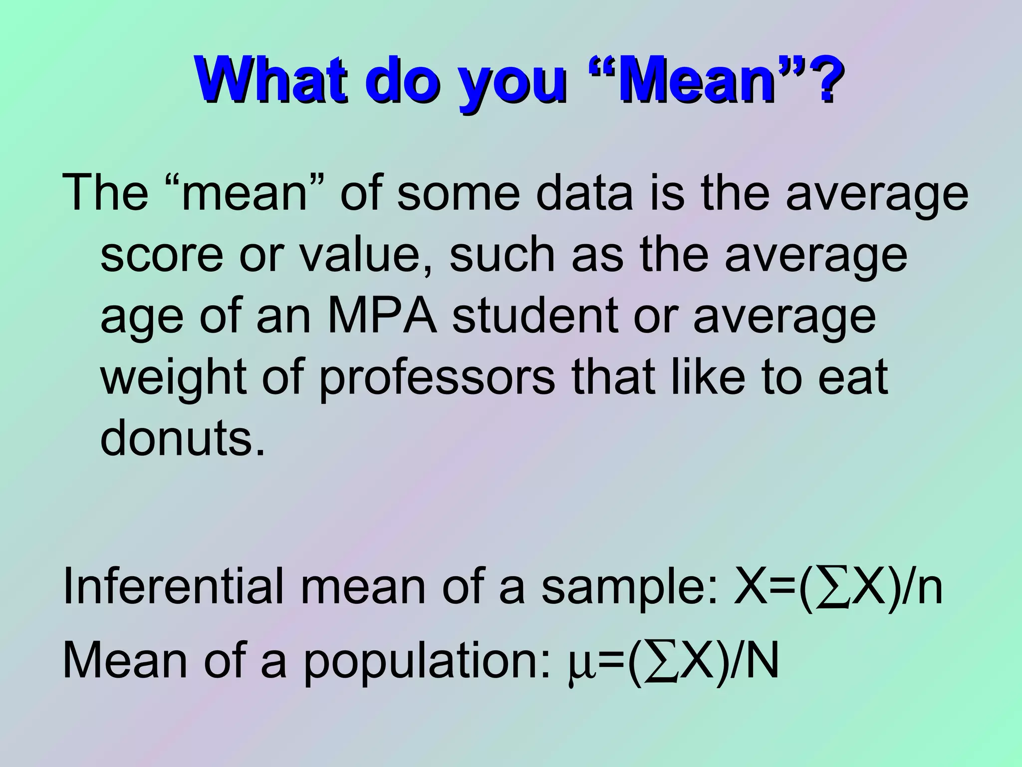
Introduction to statistics; types (descriptive, inferential); central tendency measures: mean, median, mode.
Definition and calculation of mean; issues with outliers. Explanation of median and percentiles in data.
Definition of mode; how to calculate; importance of frequency in research.
Understanding variability in data using range, standard deviation, variance, and their formulas.
Standard deviation overview; interpretation in prediction; example with probabilities.
Inputting data into Excel; organizing data, graph types (histograms, pie charts, line graphs).
Scatter plots depicting relationships in data, specifically between presidential approval and unemployment.


