lecturenote_341796756Chapter Two_sediment transport.pdf

River Engineering Chapter Two-Sediment Transport
1
WU_KIOT- WRIE
CHAPTER TWO
Sediment Transport
2.1 Introduction
 Need for Understanding of Sediment Transport in Rivers
Understanding of sediment transport processes is essential for integrated river management and
river engineering. A river is not only conveying water, but has many other functions. One of
these functions is the transport of erosion products (boulders, gravel, sand silt and clays) from
its catchment in the downstream direction. If the transport capacity of the river is affected, e.g.
by diversion of water from the river or by storing water in a reservoir, deposition of sediments
may occur. If not properly taken care of, harmful sedimentation and/or erosion may occur due
to water management measures, which then again to be remedied. Hence, good water
management (and more generally good river management, which includes also the
management of, e.g. flood plain of the river) includes sediment management. For this,
sufficient understanding of the sediment transport processes in the river is a must.
There are, however, other reasons why good understanding of sediment transport process is
indispensable. The most important ones are listed hereafter:
(a) Morphological boundary conditions for design of hydraulic structures and river
training works.
For the design of such structures boundary conditions have to be specified. These
comprise not only the discharge, maximum and minimum water levels and current
velocities, but also the lowest bed levels that may occur in a river and the future changes
in the morphological characteristics of the river (changes in the “form” of the river;
morphology is the science of the form of the river) near the structure. These levels and
possible changes are effectuated by gradients in the sediment transport rates. Changes are
not only due to natural processes like the variation of the discharge in time or ongoing
bank erosion, but there will also be an interaction between the future structure and the
nearby flow pattern and sediment transport. Also the latter should be accounted for
properly. This requires understanding of the interaction between flow, sediment and
structure.
(b) Sedimentation in Reservoirs
Many reservoirs are suffering from excessive sedimentation. Often this is due to the fact
that either the upstream sediment supply was never considered or that the seriousness of
this process was underestimated, e.g. because not sufficient data were available. Also
changes in sediment yield, e.g. due to changed land use in the upstream catchment, can
cause detrimental sedimentation. To remedy the negative effects (loss in storage capacity),
changes in the operation of the reservoir are often required, sometimes with drastic
consequences, e.g. the reduction of the power production.
(c) Sediment problems at Intakes
Many main canals of irrigation projects suffer from excessive sedimentation, which is
entering via the headworks. Often this is due to the fact that the sediment transport in the
river was not properly assessed and appears to be much larger than anticipated. Another

2
WU_KIOT- WRIE
reason is that morphological changes have taken place after construction of the intake
structure, which jeopardized the measures taken to exclude sediment when withdrawing
water. Remedial measures are rehabilitation of the intake structure or regular cleaning of
the canals, which both are very expensive.
(d) Environmental Impact Assessment
There is an increasing awareness of possible environmental impact of water management
schemes and river training works. To assess the potential impacts of such schemes not
only their hydraulic impacts should be assessed but also possible morphological changes
(degradation or aggradation, changes in flood plain sedimentation, etc) should be
identified. This assessment can only be done when sufficient understanding is available on
sediment transport processes.
Many more examples can be given which all stress the importance of understanding sediment
loads and sediment transport processes in rivers before embarking on major water management
schemes or river training.
These lecture notes attempt to provide the student with a basic understanding of sediment
transport in rivers. Necessarily it can only give an introduction to sediment transport processes.
2.2 Origin and properties of sediments
2.2.1 Introduction
The processes of erosion of land surfaces, transportation of eroded materials, deposition of this
material in lakes and reservoirs and such other processes depend on several factors. These
factors can be generally classified into the following categories: characteristics of sediment,
characteristics of the fluid, characteristics of the flow, and characteristics of the channel.
The sediment characteristics, such as its relative density, size, shape, etc play a decisive role in
various stages of the phenomenon of sediment transport and, therefore, these will be discussed
here in detail along with the methods of determining these properties. These properties are
governed to a large extent by the origin of the sediment and the process of its formation. Hence
attention will first be directed towards the origin and formation of sediments.
2.2.2 Origin and formation of sediments
All sediments transported by water and air and also those found in deserts have resulted by the
process of weathering of rocks. Weathering can be defined as the process by which solid rocks
are broken up and decayed. The size, the mineral composition, the density and other factors
such as surface texture depend on the nature of the parent rock from which the sediments are
formed. The processes of weathering can be subdivided into chemical weathering, mechanical
weathering, and organic weathering.
The three agents in the atmosphere which are responsible for chemical weathering are oxygen,
carbon dioxide and water vapour. In certain cases, carbonic acid and excess water act on
granite, albite, biotite, etc and give free silica, carbonate of alkali elements and other secondary
minerals. This process loosens the rocks of land surface and alters them to easily erodible

3
WU_KIOT- WRIE
material. Sometimes the iron ores are oxidized. In certain other cases hydration of minerals
gives rise to new secondary minerals and increases their volume.
Several mechanical agents also disintegrate the parent rocks into fragmental material. These
agents include:
 Freezing water
 Expansion caused by chemical changes
 Exfoliation resulting from sudden changes in temperature
Volume of water increases by approximately ten per cent when it freezes. When the water is
confined, such expansion causes a considerable force. Therefore, water which enters the cracks
and fissures and freezes tends to push the rock apart. Repeated freezing and thawing at high
altitude can be one of the most important disintegrating forces for the rocks. In certain cases
secondary minerals such as kaolinite formed by chemical weathering occupy a volume much
greater than the original mineral. This can create forces which ultimately break the rocks. In
some other processes called chemical exfoliation, the sheets are notably decayed and
discolored. The work performed by the solutions which penetrate slowly along the cleavage
cracks of crystals and between the grains and thereby induce the formation of new minerals of
large volumes which causes disintegration. Exfoliation or scaling also occurs due to extreme
heating followed by sudden cooling.
Organic agents of weathering are primarily burrowing animals and also roots and trunks of
trees which wedge the rocks apart.
After the parent rocks are disintegrated, the material is transported from one place to another
and deposited by streams, wind, or glaciers. The materials are called alluvium if transported
and deposited by streams, loess if transported and deposited by wind, and glacial drift if it is
transported and deposited by glaciers.
Stream erosion and deposition
The sediment load carried by streams comes from various sources. In the hilly areas the
streams pick up coarse material from the talus. (Talus is a geological term describing a heap or
sheet of coarse rock that has accumulated at the foot of the hill or on a steep slope.) Landslides
also contribute to the load carried by streams. However, the major portion of the sediment load
carried by streams comes from the erosion of material in the drainage basin; a certain amount
also originates as a result of weathering of rocks from the bed and banks of the stream. The
size of the sediment transported in any reach is dependent on the geology of the basin as well
as the distance of the reach from the source. The amount of the sediment load carried depends
on the size of materials, discharge, slope, and channel and catchment characteristics.
Wind erosion and deposition
Arid and semi-arid regions are characterized by relatively low and infrequent rainfall. As such,
stream flows in these regions are small, unless, of course, the area is small and is traversed by
stream flowing into the area from an area of appreciable rainfall. However, in general, stream
erosion in arid and semi-arid regions is relatively small.

4
WU_KIOT- WRIE
On the other hand, wind erosion becomes a predominant factor. High velocity winds, carrying
fine sand with them, are effective agents of wind erosion. When wind blows over deserts and
ploughed fields, fine sand and dust particles are carried away while the coarser material is left
behind. This process is called deflation. The dust that is carried by the wind is transported to
great distances. When the wind velocity is reduced, this material is deposited as loess.
Glacial erosion and deposition
As big pieces of ice move over land surface, they pick up loose rock, boulders, and sand along
with them. This material acts as an abrasive agent to loosen other materials and reduce the size
of this material. The transporting capacity of glaciers is large enough to transport rocks of the
size of rooms. When the glacier melts most of the materials that it has been carrying is dropped
and deposited.
2.2.3 Properties of sediment
Sediments are broadly classified as cohesive and noncohesive (or cohesionless). With cohesive
sediments, the resistance to erosion depends on the strength of the cohesive bond binding the
particles. Cohesion may far outweigh the influence of the physical characteristics of the
individual particles. On the other hand, the cohesionless sediments generally consist of larger
discrete particles than the cohesive soils. Cohesionless sediment particles react to fluid forces
and their movement is affected by the physical properties of the particles such as size, shape,
and density.
Sediment properties of individual particles that are important in the study of sediment transport
are particle size, shape, density, specific weight, and fall velocity.
Size
Size is the basic and most readily measurable property of sediment. Size has been found to
sufficiently describe the physical property of a sediment particle for many practical purposes.
The size of a particle can be determined by caliper, sieve or by sedimentation methods. The
size of an individual particle is not of primary importance in river mechanics or sedimentation
studies, but the size distribution of the sediment that forms the bed and banks of the stream or
reservoir are of great importance.
Shape
Shape refers to the geometric form or configuration of a particle regardless of its size or
composition. Corey investigated several shape factors, and concluded that from the viewpoint
of simplicity and effective correlation, the following ratio was most significant expression of
shape.
ab
c
Sp  (2.1)
In this equation, a, b, and c are the lengths of the longest, the intermediate, and the shortest
mutually perpendicular axes through the particle, respectively, and Sp is the shape factor (also
called Corey’s shape factor). The shape factor is 1.0 for sphere. Naturally worn quartz particles
have an average shape factor of 0.7.
Density

5
WU_KIOT- WRIE
The density of a sediment particle refers to its mineral composition. Usually, specific gravity,
which is defined as the ratio of specific weight or density of sediment to specific weight or
density of water, is used as an indicator of density. Waterborne sediment particles are primarily
composed of quartz with specific gravity of 2.65.
Specific weight
Specific weight is an important factor extensively used in hydraulics and sediment transport.
The specific weight of deposited sediment depends on the extent of consolidation of the
sediment. It increases with time after initial deposition. It also depends on the composition of
the sediment mixture.
Fall velocity, ω
The fall velocity, or the terminal fall velocity, that a particle attains in a quiescent column of
water, is directly related to relative flow conditions between the sediment particle and the
water during conditions of sediment entrainment, transportation, and deposition. The fall
velocity reflects the integrated result of size, shape, surface roughness, specific gravity, and
viscosity of fluid. The fall velocity of a particle can be calculated from a balance between the
particle buoyant weight and the resisting force resulting from fluid drag. The general drag
equation is
2
A
C
F
2
D
D


 (2.2)
where FD = drag force; CD = drag coefficient; ρ = density of water; A = the projected area of
particle in the direction of fall, and ω = the fall velocity.
The buoyant or submerged weight of a spherical sediment particle is
 g
r
3
4
W s
3
s 



 (2.3)
Where, r is the particle radius.
The fall velocity can be solved from equations (2.2) and (2.3) once the drag coefficient has
been determined. The drag coefficient is a function of Reynolds number and shape factor.
Theoretical consideration of drag coefficient: For a very slow and steady moving sphere in
an infinite liquid at a very small Reynolds number, the drag force can be expressed as



 r
6
FD (2.4)
The drag coefficient is then found to be (this is the viscous or Stokes range where Re is less
than 0.1)
e
D
R
24
C  (2.5)
Where, Re = Reynolds number.
Equation (2.5) is acceptable for Reynolds numbers less than 1.0.
From equation (2.2) and (2.5), Stoke’s equation can be obtained, i.e.,




 d
3
FD (2.6)
From equation (2.3) and (2.6), the terminal fall velocity for a sediment particle is

6
WU_KIOT- WRIE







2
18
1 d
g
s
(2.7)
where d is the sediment diameter.
Equation (2.7) is applicable for the estimation of fall velocity of a sediment particle in water if
the particle diameter is equal to or less than 0.1 mm. The value of kinematic viscosity in
equation (2.7) is a function of water temperature, and can be computed from
 
2
6
2
T
000221
.
0
T
0337
.
0
0
.
1
10
x
79
.
1 


 
(2.8)
where T is water temperature in °C.
Oseen included some inertia terms in his solution of the Navier-Stokes equation. The solution
thus obtained is
 
e
16
3
e
D R
1
R
24
C 
 (2.9)
Goldstein provided a more complete solution of the Oseen approximation, and the drag
coefficient becomes










 ...
R
20480
71
R
1280
19
R
1
R
24
C 3
e
2
e
e
16
3
e
D (2.10)
Equation (2.10) is valid for Reynolds number up to 2.0.
Rubey’s formula: Rubey introduced a formula for the computation of fall velocity of gravel,
sand, and silt particles. For quartz particles with diameter greater than 1 mm, the fall velocity
can be computed by
2
1
s
g
d
F 


















 (2.11)
where the parameter F= 0.79 for particles greater than 1 mm settling in water with temperature
between 10°C and 25°C, and d is the particle diameter.
For smaller grain sizes
   
 
2
1
2
1
1
d
g
36
1
)
(
d
g
36
3
2
F
s
3
2
s
3
2


























 (2.12)
For particle sizes greater than 2 mm, the fall velocity in 16°C water can be approximated by
 
m
in
d
,
s
/
m
in
d
32
.
3 2
1


 (2.13)
2.2.4 Bulk Properties of Sediment
The size distribution, specific weight, and porosity of bed material are the three important bulk
properties in the study of sediment transport.
1. Particle Size Distribution: While the properties and behavior of individual sediment
particles are of fundamental concern, the greatest interest is in groups of sediment particles.

7
WU_KIOT- WRIE
Various sediment particles moving at any time may have different sizes, shapes, specific
gravities, and fall velocities. The characteristic properties of the sediment are determined by
taking a number of samples and making a statistical analysis of the samples to determine the
mean, distribution, and standard deviation of the sample.
The most commonly used method to determine size frequency is mechanical or sieve analysis.
In general, the results are presented as cumulative – size frequency curves. The fraction or
percentage by weight of sediment that is smaller or larger than a given size is plotted against
particle size.
Usually, sediments are referred to as gravel, sand, silt or clay. These terms refer to the size of
the sediment particle. Table 2.1 presents the grain size scale of the American Geophysical
Union. This scale is based on powers of 2, which yields a linear logarithmic scale via the phi-
parameter defined as Φ = - log2d (with d in mm).
Table 2.1 Grain size scale of American Geophysical Union
Various methods are available to determine the particle size. Cobbles can be measured directly
with ruler. Gravel, sand and silt are analyzed by wet or dry sieving methods yielding sieve
diameters. Clay materials are analyzed hydraulically by using settling methods yielding the
particle fall velocity from which the standard fall diameter is computed.
A natural sample of sediment particles contains particles of a range of sizes. The size
distribution of such a sample is the distribution of sediment material by percentages of weight,
usually presented as a cumulative frequency distribution (see Figure 2.1).

8
WU_KIOT- WRIE
(a) (b)
Figure 2.1 Particle size distribution curves
The frequency distribution is characterized by:
 Median particle size – d50 which is the size at 50% by weight is finer,
 Mean particle size -   100
d
p
d i
i
m 
 , with pi = percentage by weight of each grain
size fraction, di.
 Geometric mean size – dg = (d15.9 d84.1)1/2
is the geometric mean of the two sizes
corresponding to 84.1% and 15.9% finer, respectively.
 Geometric standard deviation – σg = (d84.1/d15.9)1/2
.
 Gradation coefficient – 









9
.
15
50
50
1
.
84
d
d
d
d
G
2. Specific Weight: The specific weight of deposited sediment depends on the extent of
consolidation of the sediment. It increases with time after initial deposition. It also
depends on the composition of the sediment mixture. The consolidation of sediment is
of interest to hydraulic engineers. For example, the life of reservoirs varies as function
of deposition and consolidation. Consolidation concepts can be used to convert
sediment load, determined in units of weight, to volume of deposits in rivers, irrigation
channels, etc.
3. Porosity: Porosity is important in the determination of the volume of sediment deposit.
It is also important in the conversion from sediment volume to sediment discharge. The
following equation can be used for the computation of sediment discharge by volume
including that due to voids, once the porosity and sediment discharge by weight have
been determined, i.e.,
p
1
V
V s
t

 (2.14)
where Vt= total volume of sediment, including that due to voids, and Vs = volume of sediment
excluding that due to voids.

9
WU_KIOT- WRIE
Sediment Terminology
The science of sediment transport deals with the interrelationship between flowing water and
sediment particles. An understanding of the physical properties of water and sediment particles
is essential to our study of sediment transport. In this section, the most commonly used
terminologies are introduced; fundamental properties of water and sediment particles are also
given.
Some commonly used terms for describing the properties of water and sediment are:
3 Density: the mass per unit volume [kg/m³]. The density of water is denoted by ρ while that
of sediment is denoted by ρs.
4 Specific weight: the weight per unit volume [kN/m³]. It is denoted by γ for water γs for
sediment. The relationship between density and specific weight is
g
s
s 

 for sediment, and
g


 for water
5 Specific gravity: The specific gravity, s, is the ratio of the specific weight of a solid or a
liquid (a given material) to that of water at 4°C. The specific gravity of most common
sediments is 2.65.
6 Nominal diameter: is the diameter of a sphere having the same volume as the particle.
7 Sieve diameter: is the diameter of a sphere equal to the length of the side of a square sieve
opening through which the particle can just pass. As an approximation, the sieve diameter
is equal to the nominal diameter.
8 Fall diameter: is the diameter of a sphere that has a specific gravity of 2.65 and has the
same terminal fall velocity as the particle when each is allowed to settle alone in quiescent,
distilled water. The standard fall diameter is the fall diameter determined at a water
temperature of 24°C.
9 Fall velocity: is the average terminal settling velocity of a particle falling alone in
quiescent distilled water of infinite extent. When the fall velocity is measured at 24°C, it is
called the standard fall velocity.
10 Angle of repose: is the angle of slope formed by a given material under the conditions of
incipient sliding.
11 Porosity: is a measure of the volume of voids per unit volume of sediment, i.e. p =vv/vt ,
where p= porosity, vv = volume of voids, vt = total volume of sediment, including that due
to voids.
12 Viscosity: is the degree to which a fluid resists flow under an applied force. Dynamic
viscosity is the constant of proportionality relating the shear stress and velocity gradient,
i.e. dy
du


 , where τ is shear stress, μ is dynamic viscosity and du/dy is the velocity
gradient. Kinematic viscosity is the ratio between dynamic viscosity and fluid density, i.e. ν
= μ /ρ, ν is kinematic viscosity.
2.3 Limitations of particle motion
The amount and size of sediment moving through a river channel are determined by three
fundamental controls: competence, capacity and sediment supply.
Competence refers to the largest size (diameter) of sediment particle or grain that the flow is
capable of moving; it is a hydraulic limitation. If a river is sluggish and moving very slowly it

10
WU_KIOT- WRIE
simply may not have the power to mobilize and transport sediment of a given size even though
such sediment is available to transport. So a river may be competent or incompetent with
respect to a given grain size. If it is incompetent it will not transport sediment of the given size.
If it is competent it may transport sediment of that size if such sediment is available (that is, the
river is not supply-limited).
Capacity refers to the maximum amount of sediment of a given size that a stream can transport
in traction as bedload. Given a supply of sediment, capacity depends on channel gradient,
discharge and the calibre of the load (the presence of fines may increase fluid density and
increase capacity; the presence of large particles may obstruct the flow and reduce capacity).
Capacity transport is the competence-limited sediment transport (mass per unit time) predicted
by all sediment-transport equations, examples of which we will examine below. Capacity
transport only occurs when sediment supply is abundant (non-limiting).
Sediment supply refers to the amount and size of sediment available for sediment transport.
Capacity transport for a given grain size is only achieved if the supply of that calibre of
sediment is not limiting (that is, the maximum amount of sediment a stream is capable of
transporting is actually available). Because of these two different potential constraints
(hydraulics and sediment supply) distinction is often made between supply-limited and
capacity-limited transport. Most rivers probably function in a sediment-supply limited
condition although we often assume that this is not the case.
Much of the material supplied to a stream is so fine (silt and clay) that, provided it can be
carried in suspension, almost any flow will transport it. Although there must be an upper limit
to the capacity of the stream to transport such fines, it is probably never reached in natural
channels and the amount moved is limited by supply. In contrast, transport of coarser material
(say, coarser than fine sand) is largely capacity limited.
2.4 Incipient Motion
Particle movement will occur when the instantaneous fluid force on a particle is just larger than
the instantaneous resisting force related to the submerged particle weight and the friction
coefficient. Cohesive forces are important when the bed consist of appreciable amounts of clay
and silt particles.
The driving forces are strongly related to the local near-bed velocities. In turbulent flow
conditions the velocities are fluctuating in space and time, which make together with the
randomness of both particle size, shape and position that initiation of motion is not merely a
deterministic phenomenon but a stochastic process as well.
Incipient motion is important in the study of sediment transport, channel degradation, and
stable channel design. Due to the stochastic nature of sediment movement along an alluvial
bed, it is difficult to define precisely at what flow condition a sediment particle will begin to
move.
Let us consider the steady flow over the bed composed of cohesionless grains. The forces
acting on the grain is shown in Fig.2.2.

11
WU_KIOT- WRIE
Figure 2.2 Forces acting on a grain resting on the bed.
The driving force is the flow drag force on the grain,
Where the friction velocity u* is the flow velocity close to the bed. α is a coefficient, used to
modify u* so that αu* forms the characteristic flow velocity past the grain. The stabilizing force
can be modeled as the friction force acting on the grain.
If u*, c, critical friction velocity, denotes the situation where the grain is about to move, then the
drag force is equal to the friction force, i.e.
which can be re-arranged into
Shields parameter is then defined as
  d
g
1
s
u2
*
*


 (2.15)
We say that sediment starts to move if
c
*,
c
*,
* u
velocity
friction
critical
u
u 
or c
,
b
c
,
b
c
,
b
b u
stress
shear
bottom
critical 





or
  d
g
1
s
u
parameter
Shields
critical
2
c
*,
c
*,
c
*,
*






Fig.2.3 shows Shields experimental results, which relate τ*,c to the grain Reynolds number
defined as
(2.16)

12
WU_KIOT- WRIE
The figure has 3 distinct zones corresponding to 3 flow situations
1) Hydraulically smooth flow for 2
d
u
R n
*
e 

 .
dn is much smaller than the thickness of viscous sublayer. Grains are embedded in the
viscous sublayer and hence, τ*,c is independent of the grain diameter. By experiments it
is found τ*,c = 0.1/Re.
2) Hydraulically rough flow for Re ≥ 500.
The viscous sublayer does not exist and hence, τ*,c is independent of the fluid viscosity.
τ*,c has a constant value of 0.06.
3) Hydraulically transitional flow for 2 ≤ Re ≤ 500.
Grain size is the same order as the thickness of the viscous sublayer. There is a
minimum value of τ*,c of 0.032 corresponding to Re = 10.
Note that the flow classification is similar to that of the Nikurase pipe flow where the bed
roughness ks is applied instead of dn.
Figure 2.3 The Shields diagram giving τ*,c as a function of Re (uniform and cohesionless
grain).
2.5 Transportation mechanisms
The sediment load of a river is transported in various ways although these distinctions are to
some extent arbitrary and not always very practical in the sense that not all of the components
can be separated in practice:
1. Dissolved load
2. Suspended load

13
WU_KIOT- WRIE
3. Intermittent suspension (saltation) load
4. Wash load
5. Bed load
Dissolved Load
Dissolved load is material that has gone into solution and is part of the fluid moving through
the channel. Since it is dissolved, it does not depend on forces in the flow to keep it in the
water column.
The amount of material in solution depends on supply of a solute and the saturation point for
the fluid. For example, in limestone areas, calcium carbonate may be at saturation level in river
water and the dissolved load may be close to the total sediment load of the river. In contrast,
rivers draining insoluble rocks, such as in granitic terrains, may be well below saturation levels
for most elements and dissolved load may be relatively small. Obviously, the dissolved load is
also very sensitive to water temperature and other things being equal, tropical rivers carry
larger dissolved loads than those in temperate environments. Dissolved loads for some of the
world’s major rivers are listed in table 2.2.
Dissolved load is not important to the geomorphologist concerned with channel processes
because it is simply part of the fluid. On the other hand, dissolved load is very important to
geomorphogists concerned with sediment budgets at a basin scale and with regional denudation
rates. In many regions most of the sediment is removed from a basin in solution as dissolved
load and must be accounted for in estimating erosion rates.

14
WU_KIOT- WRIE
Table 2.2 Sediment loads of major world rivers (after Knighton, 1998: Figure 3.2). Sources: Degens et al (1991),
Meybeck (1976) and Milliman and Meade (1983).
Suspended-sediment load
Suspended-sediment load is the clastic (particulate) material that moves through the channel in
the water column. These materials, mainly silt and sand, are kept in suspension by the upward
flux of turbulence generated at the bed of the channel. The upward currents must equal or
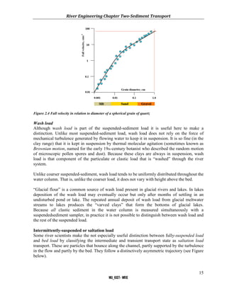
exceed the particle fall-velocity (Figure 2.4) for suspended-sediment load to be sustained.

15
WU_KIOT- WRIE
Figure 2.4 Fall velocity in relation to diameter of a spherical grain of quartz
Wash load
Although wash load is part of the suspended-sediment load it is useful here to make a
distinction. Unlike most suspended-sediment load, wash load does not rely on the force of
mechanical turbulence generated by flowing water to keep it in suspension. It is so fine (in the
clay range) that it is kept in suspension by thermal molecular agitation (sometimes known as
Brownian motion, named for the early 19th-century botanist who described the random motion
of microscopic pollen spores and dust). Because these clays are always in suspension, wash
load is that component of the particulate or clastic load that is “washed” through the river
system.
Unlike coarser suspended-sediment, wash load tends to be uniformly distributed throughout the
water column. That is, unlike the coarser load, it does not vary with height above the bed.
“Glacial flour” is a common source of wash load present in glacial rivers and lakes. In lakes
deposition of the wash load may eventually occur but only after months of settling in an
undisturbed pond or lake. The repeated annual deposit of wash load from glacial meltwater
streams to lakes produces the “varved clays” that form the bottoms of glacial lakes.
Because all clastic sediment in the water column is measured simultaneously with a
suspendedsediment sampler, in practice it is not possible to distinguish between wash load and
the rest of the suspended load.
Intermittently-suspended or saltation load
Some river scientists make the not especially useful distinction between fully-suspended load
and bed load by classifying the intermediate and transient transport state as saltation load
transport. These are particles that bounce along the channel, partly supported by the turbulence
in the flow and partly by the bed. They follow a distinctively asymmetric trajectory (see Figure
below).

16
WU_KIOT- WRIE
Figure 2.5 The trajectory of saltating (intermittentlysuspended) sediment grains moving in the flow
Saltation load may be measured as suspended load (when in the water column)
or as bed load (when on the bed). Although the distinction between saltating load and
other types of sediment load may be important to those studying the physics of
grain movement, most geomorphologists are content to ignore it as a special case.
Bed Load (Traction Load)
Bed load is the clastic (particulate) material that moves through the channel fully supported by
the channel bed itself. These materials, mainly sand and gravel, are kept in motion (rolling and
sliding) by the shear stress acting at the boundary. Unlike the suspended load, the bed-load
component is almost always capacity limited (that is, a function of hydraulics rather than
supply). A distinction is often made between the bed-material load and the bed load.
Bed-material load is that part of the sediment load found in appreciable quantities in the bed
(generally > 0.062 mm in diameter) and is collected in a bed-load sampler. That is, the bed
material is the source of this load component and it includes particles that slide and roll along
the bed (in bed-load transport) but also those near the bed transported in saltation or
suspension. The material eroded from the river bed, referred to as bed-material load, is transported by
the river as bed load and as suspended load. Coarse sediment (cobbles, grave and coarse sand) is
normally transported by the flow as bed load, close to the bed surface. Fine material (medium and
fine sand) is transported in suspension. It is kept in suspension by the water turbulence for a
distance that depends on the fall velocity of the grain
Bed load, strictly defined, is just that component of the moving sediment that is supported by
the bed (and not by the flow). That is, the term “bed load” refers to a mode of transport and not
to a source.
2.6 Bed forms and Bed Roughness
Bedforms are relief features initiated by the fluid oscillations generated downstream of small
local obstacles over a bottom consisting of movable (alluvial) sediment materials. Once
sediment starts to move, various bedforms occur.
Classification of Bed forms
1. Bedforms in Sand-bed Rivers

17
WU_KIOT- WRIE
Many types of bedforms can be observed in nature. When the bedform crest is perpendicular
(transverse) to the main flow direction, the bedforms are called transverse bedforms, such as
ripples, dunes and anti-dunes (see Fig. 3.4). Ripples have a length scale smaller than the water
depth, whereas dunes have a length scale much larger than the water depth. Figure 3.4 shows
the various bedforms observed in rivers.
Ripples and dunes travel downstream by erosion at the upstream face (stoss side) and
deposition at the downstream face (lee side). Antidunes travel upstream by lee side erosion and
stoss side deposition (see Figure 2.6).
Bedforms with their crest parallel to the flow are called longitudinal bedforms such as ribbons
and ridges. In laboratory flumes the sequence of bedforms with increasing flow intensity is
Plane (flat) bed: is a plane bed surface without elevations or depressions larger than the
largest grain of the bed material.
Ripples: Ripples are formed at relatively weak flow intensity and are linked with fine
materials, with d50 less than 0.7 mm. The size of ripples is mainly controlled by grain size. By
observations the typical height and length of ripples are
At low flow intensity the ripples have a fairly regular form with an upstream slope 6° and
downstream slope 32°. Ripple profiles are approximately triangular, with long gentle upstream
slopes and short, steep downstream slopes.
Dunes: The shape of dunes is very similar to that of ripples, but it is much larger. The size of
dunes is mainly controlled by flow depth. Dunes are linked with coarse grains, with d50 bigger
than 0.6 mm. With the increase of flow intensity, dunes grow up, and the water depth at the
crest of dunes becomes smaller. It means a fairly high velocity at the crest, dunes will be
washed-out and the high stage flat (plane) bed is formed.
Transition: This bed configuration is generated by flow conditions intermediate between those
producing dunes and plane bed. In many cases, part of the bed is covered with dunes while a
plane bed covers the remainder.
Antidunes: These are also called standing waves. When Froude number exceeds unity
antidunes occur. The wave height on the water surface is the same order as the antidune height.
The surface wave is unstable and can grow and break in an upstream direction, which moves
the antidunes upstream.
Bars: These are bed forms having lengths of the same order as the channel width, or greater,
and heights comparable to the mean depth of the generating flow. These are point bars,
alternate bars, middle bars, and tributary bars.

18
WU_KIOT- WRIE
Chutes and Pools: These occur at relatively large slopes with high velocities and sediment
concentrations.
2. Bed forms in Gravel-bed Rivers
The bed materials of gravel-bed rivers usually have a broad range of grain sizes from sand
particles to large boulders. As a result, selective transport processes and armouring of the bed
surface may occur locally. The most common regime is the lower transport regime; the
transition regime (with plane bed) is a rare event. Very regular bed-features such as mega-
ripples and dunes have been observed in laboratory flumes and small-scale channels. Various
types of three-dimensional bar forms (referred to as alternate bars, crescent bars, transverse
bars, deltaic bars) have been observed in depositional regions of rivers (see Fig. 2.8).
Figure 2.6 Bed form types in rivers

19
WU_KIOT- WRIE
Figure 2.7 Bed form migration in lower and upper regimes
Figure 2.8 Three-dimensional large-scale bar forms
2.7 Bed Load, Suspended Load, Wash Load and Total Load Transport
General
When the values of the bed shear velocity just exceeds the critical value for initiation of
motion, the bed material particles will be rolling and/or sliding in continuous contact with the
bed. For increasing values of the bed shear velocity the particles will be moving along the bed
by more or less regular jumps, which are called saltations.
When the value of the bed shear velocity begins to exceed fall velocity of the particles, the
sediment particles can be lifted to a level at which the upward turbulent forces will be of
comparable or higher order than the submerged weight of the particles and as a result the
particles may go into suspension.

20
WU_KIOT- WRIE
Usually, the transport of particles by rolling, sliding and saltating is called bed load transport,
while the suspended particles are transported as suspended load transport. The suspended load
may also include the fine silt particles brought into suspension from the catchment area rather
than from the streambed material (bed material load) and is called the wash load. A grain size
of 63 μm (dividing line between silt and sand) is frequently used to separate between bed
material and wash load.
Bed load and suspended load may occur simultaneously, but the transition zone between both
modes of transport is not well defined.
The following classification and definitions are used for the total sediment transported in
rivers.
2.7.1 Bed Load Transport
Usually, the transport of particles by rolling, sliding and saltating is called the bed load
transport. Saltation refers to the transport of sediment particles in a series of irregular jumps
and bounces along the bed (see Figure 2.9).

21
WU_KIOT- WRIE
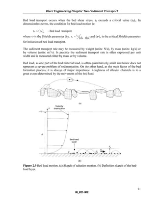
Bed load transport occurs when the bed shear stress, τ0 exceeds a critical value (τ0)c. In
dimensionless terms, the condition for bed-load motion is:
  transport
load
Bed
c
*
* 



where τ* is the Shields parameter (i.e.  
 
gd
1
s
0
* 



 and (τ*)c is the critical Shields parameter
for initiation of bed load transport.
The sediment transport rate may be measured by weight (units: N/s), by mass (units: kg/s) or
by volume (units: m3
/s). In practice the sediment transport rate is often expressed per unit
width and is measured either by mass or by volume.
Bed load, as one part of the bed material load, is often quantitatively small and hence does not
represent a severe problem of sedimentation. On the other hand, as the main factor of the bed
formation process, it is always of major importance. Roughness of alluvial channels is to a
great extent determined by the movement of the bed load.
Figure 2.9 Bed load motion. (a) Sketch of saltation motion. (b) Definition sketch of the bed-
load layer.

22
WU_KIOT- WRIE
Bed Load Formulae
Various formulas are developed in the past for estimation of bed load discharge. Estimates of
bed load transport using different formula for the same set of given data are also found to give
widely different results. Here, only few of the most common formulae and approaches are
presented.
1. Discharge Approach (bed load expressed in terms of discharge)
This approach, relating the quantity of transported sediment to water discharge, had been one
of the main approaches adopted before the notion of shear stress gained prominence in later
years. Main formulae of this kind are those proposed by Schoklitsch, Meyer-Peter and Casey,
etc.
Schoklitsch Formula (1934 & 1943)
The stream is supposed to be wide, hence the sediment discharge relates to unit width of the
bed. The main empirical relation reads as
 
c
b q
q
d
S
7000
q
2
1
2
3

 (2.17a)
where qb= bed load (kg/s/m), d = grain size (mm), S = energy slope, q = specific water
discharge (m³/s/m), qc= critical discharge (m³/s/m).
The critical water discharge, i.e. the discharge that causes incipient motion, for sediments with
specific gravity 2.65 is given by
3
4
S
d
10
x
94
.
1
q 5
c

 (2.17b)
The 1943 Schoklitsch formula is
 
c
b q
q
S
2500
q 2
3

 (2.18a)
For sediments with specific gravity 2.65, the critical discharge in eq (2.18a) is given by
6
7
2
3
S
d
6
.
0
qc  (2.18b)
Equations (2.17) and (2.18) have been developed for uniform grain distributions. It is,
however, generally applied to non-uniform distributions also, taking d50 (median size) as the
characteristic diameter for the mixture. Schoklitsch also suggested a more accurate method,
which is as follows:
Sediment mixture is arbitrarily subdivided into several size sub-ranges having mean
diameters da, db, dc, etc; and the partial quantity of each sub-range is then determined
and expressed as percentage of the total quantity. Subsequently, partial bed loads qba,
qbb, qbc, etc. are computed for each mean diameter for the given discharge, q, and given
slope, S, using equations (2.17 and 2.18). The total bed load for the sediment mixture is
then obtained,
qb = a qba +b qbb + c qbc + …
where a, b, c, … indicate the percentage quantities that each partial sub-range is of the
total.
This formula is applicable to grain sizes in the range of 0.3 – 7.0 mm.
2. Shear Stress Approach

23
WU_KIOT- WRIE
This approach is much more favored today, because of the importance accorded to the shear
stress in all aspects of the sediment movement in alluvial channels. Formulae of this type are
those of Straub-Du Boys, Shield, Kalinske, Meyer-Peter and Mueller, etc.
The best known of these, and probably the most widely used, is the Meyer-Peter and Mueller
formula; it also gives the best agreement with measured data.
The maximum amount of sediment that is transported by the river as bed-material load can be
related to the stream velocity and is called sediment transport capacity. Therefore, the transport
of material eroded from the riverbed is capacity limited, which means that a certain current
cannot transport more sediment than a certain amount, even when this is available on the river
bed.
In alluvial bed rivers, the bed-material load can be assumed to be always equal to the sediment
transport capacity. This is not true, however, for rivers that are not fully-alluvial, i.e. those rivers
characterized by rock outcrops or armoured bed. For semi-alluvial rivers the amount of bedmaterial
load is generally smaller than the sediment transport capacity, because of the limited
availability of sediment from the bed. All transport capacity formulas have been derived from
laboratory experiments and include empirical features. A relevant consequence is that all
morphodynamic predictions that are based on sediment transport formulas have an empirical
character and are not exact. The general sediment transport capacity formula has the form:
(2.19)
where qS is the amount of bed-material load per meter of river width (m2
/s); m is a
proportionality coefficient, u is the local stream velocity; uc is the critical value of velocity
below which no sediment transport occurs; b is the exponent (values always larger than 3).
The best formula is always the one that was derived for flow and sediment conditions that are
similar to the case under study. In general, the presence of a threshold for sediment motion (for
instance uc in Equation above) is important for coarse sand, gravel and large sediment
particles. It is less relevant for fine sand, which is almost always mobilized by river flows.
Meyer-Peter and Mueller Formula
A commonly used formula for gravel-bed rivers is the one derived by Meyer-Peter & Müller
(1948). This formula (MPM) is restricted to bed load capacity, since the conditions for which it
was derived did not present much transport in suspension::
(2.20)
where

24
WU_KIOT- WRIE
The sediment transport formula computes the volume of sediment (bed-material load)
transported per unit of time and per metre of river width, in m2
/s. If this volume includes an
extra 40% occupied by pores (sand): KMPM = 13.3. If the volume does not include the volume
occupied by pores: KMPM = 8. Wong and Parker (2008) recently corrected the value of KMPM.
According to them, KMPM = 6.65 (with pores) and KMPM = 4 (without pores). They also suggest
imposing  1 if bedforms (dunes) are absent.
Unlike Engelund & Hansen, the Meyer-Peter & Müller formula includes a threshold. If  
0.047 no sediment transport occurs. Thus   0.047 represents Meyer-Peter & Müller’s
condition for initiation of motion. This threshold is not coincident with the Shield’s threshold,
because it was derived from other experimental data. The MPM threshold is valid only for the
experiments carried out by Meyer-Peter & Müller and for river channels satisfying the criteria
for the application of the formula:
This equation shows that the exponent b varies with the stream velocity and is high close to the
conditions of initiation of motion. Values of b approaching 3 reflect conditions of high
sediment mobility in which sediment is partly moving in the water column.
Shields Formula
The semi-empirical formula derived by Shields for a level bed is
 
 d
S
q
10
q
s
s
c
b








 (2.21)
where d = d50 , and S = bed slope.
In this formula τ and τc can be calculated from
  50
s
c gd
056
.
0 



 and
S
R
g



Equation (2.21) is dimensionally homogeneous, and can be used for any system of units. The
critical shear stress can also be obtained from Shields diagram.

25
WU_KIOT- WRIE
2.7.2 Suspended Load Transport
Suspended load refers to sediment that is supported by the upward components of turbulent
currents and stays in suspension for an appreciable length of time. In most natural rivers,
sediments are mainly transported as suspended load.
The suspended load transport can be defined mathematically as


h
a
sv dz
c
u
q (2.22a)



h
a
s
sw dz
c
u
q (2.22b)
where qsv and qsw are suspended load transport rates in terms of volume and weight,
respectively; c
and
u are time averaged velocity and sediment concentration, by volume at a
distance z above the bed, respectively; a is thickness of the bed load transport; and h is the
water depth.
Before eq. (2.22) is integrated, c
and
u must be expressed mathematically as a function of z.
Under steady equilibrium conditions, the downward movement of sediment due to the fall
velocity must be balanced by the net upward movement of sediment due to turbulent
fluctuations, i.e.,
0
dz
dC
C s 


 (2.23)
where εs is the momentum diffusion coefficient for sediment, which is a function of z; ω is fall
velocity of sediment particles; and C is sediment concentration.
For turbulent flow, the turbulent shear stress can be expressed as
dz
du
m
z 


 (2.24)
where εm is kinematic eddy viscosity of fluid or momentum diffusion coefficient for fluid.
It is generally assumed that
m
s 


 (2.25)
where β is a factor of proportionality.
For fine sediments in suspension, it can be assumed that β = 1 without causing significant
error. Eq.(2.23) can also be written as
0
dz
C
dC
s



 (2.26)
and integration of eq.(3.43) yields











 
z
a s
a
dz
exp
C
C (2.27)

26
WU_KIOT- WRIE
where C and Ca are sediment concentrations by weight at distance z and a above the bed,
respectively.
The shear stress at a distance z above the bed is
  












h
z
1
z
h
S
z (2.28)
where τ and τz are shear stresses at channel bottom and a distance z above the bed,
respectively.
Assume the Prandtl – von Karman velocity distribution is valid, i.e.,
z
k
U
dz
du *
 (2.29)
From equations (2.24), (2.28) and (2.29),
)
z
h
(
h
z
U
k *
m 

 (2.30)
and )
z
h
(
h
z
U
k *
s 


 (2.31)
Equation (2.30) indicates that εm =0 at z = 0 and z =h. The maximum value of εm occurs at z =
½ h.
On substituting eq. (2.31) into eq. (2.26) and integration from a to z, assuming β = 1, yields
Z
a a
h
a
z
z
h
C
C








 (2.32)
where
*
U
k
Z

 is known as the Rouse constant and equation (2.32) is called the Rouse
equation. This equation gives the distribution of the suspended sediment concentration over the
vertical for various values of Z (see Fig. 2.10).
Figure 2.10 Suspended sediment distributions according to equation (2.32)

27
WU_KIOT- WRIE
2.7.3 Wash load
Silt and clay that is transported by river flows mainly originates from soil erosion (due to rain,
landslides, debris and mud flows) and from the falling of cohesive river banks. This material is
transported as suspended load. It is kept in suspension by the water turbulence and since the
fall velocity is very small, it does not settle in the river main channel, but flows downstream
until it reaches a lake, a reservoir or the estuary. It is called wash load. The amount of material
transported as wash load is supply limited, which means that the amount of this very fine
material travelling with the water is generally limited by its input and not by the capacity of the
current to transport it. Extreme high concentrations of fine sediment might transform the water
flow into a mud flow. In general, there is no quantitative relation between flow velocity and
wash load, except from some specific cases, although the highest amounts of wash load often
occur during floods. This means that the amount of wash load cannot be determined as a
function of the flow characteristics, such as flow velocity. It has to be determined by other
means, i.e. from soil erosion rates or by measuring suspended solid concentrations for long
periods of time.
High concentrations of sediment flowing on steep slopes (steepeness higher than 15%) are
called debris flows. This sediment is a mixture of large and small sediment grains. If a debris
flow reaches the valley and enters the river bed, where the slope is much gentler, most of the
largesized material settles and only a limited part is transported by the river current as bed load
(capacity limited), while the very fine material continues its journey to the sea as wash load.
Organic sediment transport is fundamentally different from inorganic transport. Organic
particles have low specific density, with relative density in water close to unit, and surface
area-to-volume ratios that is higher than inorganic sediments. Besides, organic material can
degrade into soluble products. Relationships between organic sediment concentration and
discharge vary considerable among watersheds due to differences in their sources of organic
materials. Large rivers with relatively long flood pulses receive important inputs of organic
matter from their floodplains as they sweep back and forth across the aquatic-terrestrial
transition zone during floods.
2.7.4 Total Load Transport
Based on the mode of transportation, total load is the sum of bed load and suspended load.
Based on the source of material being transported, total load can also be defined as the sum of
bed material load and wash load. Wash load consists of fine materials that are finer than those
found in the bed. The amount of wash load depends mainly on the supply from the watershed,
not on the hydraulics of the river. Consequently, it is difficult to predict the wash load based on
the hydraulic characteristics of a river. Most total load equations are, therefore, totals bed
material load equations.
General Approaches
There are two general approaches to the determination of total load:
(1) Computation of bed load and suspended load separately and then adding them together to
obtain total load – indirect method, and
(2) Determination of total load function directly without dividing it into bed load and
suspended load – direct method.

28
WU_KIOT- WRIE
Engelund & Hansen (bed + suspended bed material loadtotal load)
This formula provides the total load thus, direct method. A commonly used sediment transport
capacity formula is the one designed by Engelund & Hansen (1967), which is valid for sand-
bed rivers only. According to Engelund & Hansen b = 5 and uc = 0; m is given by the
following expression:
(2.33)
The sediment transport formula computes the volume of sediment (bed-material load)
transported per unit of time and per metre of river width, in m2
/s. If the volume of sediment
includes also an extra 40%, i.e. the volume occupied by the pores between the grains (sand):
KEH = 12. If the volume does not include pores: KEH =20. The sediment balance equation,
which is necessary to compute the bed level changes in a specific reference area, will have to
take into account whether the adopted sediment transport formula includes pores or not.
The sediment transport formula of Engelund & Hansen was derived from cases in which
sediment (sand) was transported as bed and suspended load. Wash load is not taken into
account. This formula can be applied to sediments and flows fulfilling the following criteria:

lecturenote_341796756Chapter Two_sediment transport.pdf

More Related Content

Similar to lecturenote_341796756Chapter Two_sediment transport.pdf

More from BedassaDessalegn3

Recently uploaded

lecturenote_341796756Chapter Two_sediment transport.pdf