PC Software - Computer Application - Office Automation Tools

A book By Mr. Ashish Patel
(Software Engineer and Professor and CEO at SAPTRSI)
Page 1

INDEX
1. Introduction
1.1. Basic DOS Commands
1.2. Concept of Windows, Icon, Menu
1.3. Desktop
1.4. Creating Folders and Shortcuts
1.5. Finding Files & Folders
1.6. Creating, Copying, Moving and Deleting files
1.7. Windows Explorer
2. Word Processing Package
2.1. Typing, Editing, Proofing & reviewing
2.2. Formatting text & Paragraph
2.3. Automatics Formatting and Styles
2.4. Working with Tables
2.5. Graphics and Frames
2.6. Mail Merge
2.7. Automating Your Work & printing documents
3. Spreadsheet package
3.1. Concept of worksheet
3.2. Working & Editing in Workbooks
3.3. Creating Formats & Links
3.4. Protecting and Hiding data
3.5. Built in Functions
3.6. Formatting a Worksheet & Creating graphics objects
3.7. Creating Charts (Graphics), Formatting and analyzing data
3.8. Organizing Data in a List (Data Management)
3.9. Sharing & Importing Data
3.10. Printing
3.11. Macros
4. Presentation Package
4.1. Creating and Editing Slides
4.2. Creating and Editing objects in the slide
4.3. Animation and Running Slide Show
4.4. Creating and Running Slide Show
4.5. Templates
4.6. Interface with other packages
5. Internet
5.1. Concepts
5.2. Working
5.3. Mailing & surfing tools
Page 2

MS - DOS (Microsoft Disk Operating System)
® MS-DOS is an operating system designed for the IBM PC by Microsoft in 1981.
® The first personal computer version of DOS, called PC-DOS, was developed for IBM
by Bill Gates and his new Microsoft Corporation. He retained the rights to market a
Microsoft version, called MS-DOS.
® MS DOS is Microsoft Disk Operating System. It is a text based OS.
® It was a command-line interface, meaning the user had to type in commands to use it,
unlike Windows which is a Graphical User Interface.
® MS DOS commands were either stored as individual programs, known as external
commands, or in a file called Command.com, which stored more commonly used
commands. These were called internal commands.
® Included in these would have been commands like COPY, DEL, DIR, CD and RD.
COPY enabled the copying of files.
DEL deleted files.
DIR gave a listing of files in a directory (now called a folder).
CD changed from one directory to another.
RD removed a directory.
 AUTOEXE.BAT:
® AUTOEXE.BAT is a system file found originally on DOS-type operating system.
® It is a plain text batch file that is located in the root directory of the boot device.
® The name of the file is an abbreviation of “automatic execution” , which describes its
function in automatically executing commands on system startup.
® AUTOEXE.BAT is most often used to set environment variables such as keyboard,
soundcard, printer and temporary file locations.
 COMMAND.COM:
® It is the filename of the default operating system shell for DOS Operating systems
and the default command line interpreter on Windows 95, Windows 98 and Windows
ME.
® It has an additional role as the first program run after boot, hence being responsible
for setting up the system by running the AUTOEXE.BAT configuration file, and
being the ancestor of all processes.
® COMMAND.COM’s successor on OS/2 and Windows NT-based operating system is
cms.exe (Command Prompt).
® COMMAND.COM has two distinct modes of work. First is the “interactive mode”,
in which the user types commands which are then executed immediately. The second
is the “batch mode”, which executes a predefined sequence of commands stored as a
text file with the extension .BAT.
Page 3

DOS Commands:
Internal Commands External Commands
BREAK
CALL
CHCP
CHDIR(CD)
CLS
COPY
CTTY
DATE
DEL(ERASE)
DIR
ECHO
EXIT
FOR
GOTO
IF
MKDIR(MD)
PATH
PAUSE
PROMPT
REM
RENAME(REN)
RMDIR(RD)
SET
SHIFT
TIME
TYPE
VER
VERIFY
VOL
APPEND.EXE
ASSIGN.COM
ATTRIB.EXE
BACKUP.EXE
CHKDSK.EXE
COMMAND.COM
COMP.EXE
DEBUG.EXE
DISKCOMP.COM
DISKCOPY.COM
DOSKEY.COM
DOSSHELL.COM
EDIT.COM
EDLIN.EXE
EMM386.EXE
EXE2BIN.EXE
EXPAND.EXE
FASTOPEN.EXE
FC.EXE
FDISK.EXE
FORMAT.COM
GRAFTABLE.COM
GRAPHICS.COM
HELP.EXE
JOIN.EXE
KEYB.COM
LABEL.EXE
MEM.EXE
MIRROR.COM
MODE.COM
MORE.COM
NLSFUNC.EXE
PRINT.EXE
QBASIC.EXE
RECOVER.EXE
REPLACE.EXE
RESTORE.EXE
SETVER.EXE
SHARE.EXE
SORT.EXE
SUBST.EXE
SYS.COM
TREE.COM
UNDELETE.EXE
UNFORMAT.COM
XCOPY.EXE
DOS Commands
1. Dir
® The dir command allows you to see the available files in the current and/or parent
directories.
Syntax:
Dir [drive:][path][filename][/p][/w][/A:Attributes][/O:order][/S][/L]
Where,
[drive:][path][filename]: Specifies drive, directory, and/or files to list.
/P: Pauses after each screenful of information
/W: uses wide list format
/A: Attributes:
H | -H : Hidden (or not hidden ) files
S | -S : System (or non system) files
D | -D : Directories (or files only).
R | -R : Read-only (or read/write) files
A | -A : Archivable (or already archives) files
/O:order:
N | -N : By name (alphabetical or reverse alphabetical)
Page 4

E | -E: By extension (alphabetical or reverse alphabetical)
D | -D: By date and time (chronologically or reverse)
S | -S: By size (increasing or decreasing)
C | -C: Sorts by Double Space compression ratio lowest to highest or highest to
lowest (version 6.0 only)
G | -G : Group directories( before, or after) other files.
/S: Displays files in specified directory and all subdirectories.
/L: uses lowercase.
Example:
® Dir
Lists all files and directories in the directory that you are currently in.
® Dir /s
Lists the files in the directory that you are in and all sub directories after that
directory, if you are at root “C:>” and type this command this will list to you every
file and directory on the C: drive of the computer.
® Dir /p
If the directory has a lot of files and you cannot read all the files as they scroll by
you can use this command and it will display all files one page at a time.
® Dir > myfile.txt
Takes the output of dir and re-routes it to the file myfile.txt instead of outputting it
to the screen.
2. Md / mkdir
Allows you to create your own directories in MS-DOS.
Syntax:
MKDIR [drive:]path OR MD [drive:]path
Examples:
® md test
He above example creates the “test” directory (folder) in the directory you are
currently in
® md c:test
Create the “test” directory in c: drive.
3. Rd / rmdir
Removes empty directories in MS-DOS.
Syntax:
RMDIR [drive:]path OR RD [drive:] path
Examples:
Page 5

® rmdir c:test
removes the test directory, if empty.
4. Cd
CD (Change Directory) is a command used to switch directories in MS-DOS.
Syntax:
CHDIR [drive:][path] OR CD[drive][path]
CHDIR[..] CD[..]
Examples:
® cd
Goes to the highest level, the root of the drive.
® cd..
goes back one directory. For example, if you are within C:WindowsCommand >
directory, this would take you to C:Windows >
Windows 95,98 and later versions have a feature in the CD command that allows
you to go back more than one directory when using the dots. For example, typing:
cd… with three dots after the cd would take you back two directories.
® cd
Typing cd alone will print the working directory. For example, if you are in
c:windows> and you type the cd it will print c:windows. For those users who
are
familiar with Unix/Linux this could be thought of as doing the pwd (print
working
directory) command.
 FILE MANAGEMENT COMMANDS
5. Copy
Allows user to copy one or more files to an alternate location.
Syntax:
Copy source [destination]
Examples:
® Copy *.* a:
Copy all files in the current directory to a: drive
6. Del / erase
Page 6

Del(erase) is a command used to remove files from your computer’s hard disk and
or other writable media.
Syntax:
DEL [drive:][path]filename[/P] OR ERASE [drive:][path]filename [/P]
Where,
[drive:][path]filename: specifies the files(s) to delete. Specify multiple files by using
wildcards.
/P: prompts for confirmation before deleting each file.
Example:
® Erase c:windows*.FAK
Delete any files that end with the FAK extension.
® Del c:windowstemp?est.tmp = (? is a single wild character for one letter).
This command would delete any file ending with est.tmp such as pest.tmp or
zest.tmp….
7. Copy con
To create a new file
Syntax:
copy con [filename]
Example:
® Copy con test.txt
A user can create a file using the copy con command as shown above, which
creates the test.txt file. Once the above command has been typed in, a user
could type in whatever he or she wishes. When you have completed creating the
file, you can save and exit the file by pressing ctrl + z, which would create ^Z,
and then press enter. An easier way to view and edit files in MS-DOS would be
to use edit command.
8. Ren / rename
Uses to rename files and directories from the original name to a new name.
Syntax:
Renames a file/directory or files/directories
RENAME [drive:][path][directoryname1][filename1][directoryname2][filename2]
OR
REN[drive:][path][directoryname1][filename1][directoryname2][filename2]
Examples:
® rename c:chope hope
Page 7

rename the directory chope to hope.
® Rename *.txt *.bak
Renames all text files to files with .bak extension.
® Rename *1_
Rename all files to begin with 1_. The asterisk (*) in this example is an example
of a wild character; because nothing was placed before or after he first asterisk,
this means all files in the current directory will be renamed with a 1_ in front of
the file. For example if there was a file named hope.txt it would be renamed to
1_pe.txt.
 GENERAL COMMAND
9. Type
Allows the user to see the contents of a file.
Syntax:
Type [drive:][path]filename
Examples:
® Type c:autoexec.bat
This would allow you to look at the autoexec.bat
10. Date
The date command can be used to look at the current date of the computer as well as
change the date to an alternate date.
Syntax:
DATE [date]
Type DATE without parameters to display the current date setting and a prompt for
a new one, press enter to keep the same date.
Examples:
® Date
Display the current date and prompt for a new one. If no date is entered the
current date will be kept.
11. Time
Allows user to view and edit the computer’s time
Syntax:
TIME[time]
Type time with no parameters to display current time setting and a prompt for a new
one. Press enter to keep the same time
Examples:
Page 8

® Time 12:00
Set the time to 12:00
12. Cls
Cls is a command that allows a user to clear the complete contents of the screen and
leave only a prompt.
Syntax:
CLS
Examples:
® Cls
Running the cls command at the command prompt would clear your screen of
all previous text and only return the prompt.
13. Ver
Displays the versions of MS-DOS (operating system)
Syntax:
VER
Examples:
® Ver
Display what version of MS-DOS or windows command prompt you’re using.
Below is an example of what this may look like.
Microsoft Windows XP [version 5.1.2600]
14. Edit
Edit allows you to view, create and/or modify their computer files.
Syntax:
Edit FileName
Examples:
® Edit c:user.txt
This would look at the user.txt. However, if the file is not found , you will have a
blank blue screen , when editing this or any file, ensure that you know what you
are placing in the files improperly editing the file can cause issues with your
computer.
Using edit you can also create files; for example, if you wanted to create a file
called myfile.txt, you would type: edit myfile.txt this would bring up a blank
blue screen , as long as the file is saved upon exit, this will create the file
myfile.txt.
15. Print
This command allowed users to print a text file to a line printer, in the background.
Page 9

Syntax:
Print filename
® Examples:
print c:file.txt
16. Format
It is used to erase all of the information off of a computer diskette or fixed drive
When using the format command, remember all information on the drive you wish
to format will be completely erased,
Syntax:
Format drive
Examples:
® Format c: /q
Quickly erases the contents of a C: drive.
17. Unformat
Used to unformat a drive that has been formatted,
Syntax:
UNFORMAT drive:
Examples:
® Unformat c:
Command specified to unformat drive c: if it was unformatted.
18. More
Allows information to be displayed one page at a time
Syntax:
Command-name | MORE [drive:][path][filename]
Where,
[drive:][path][filename] : Specifies file(s) to display one screen at a time.
Command-name : specifies a command whose output will be displayed.
Examples:
® Dir | more
Allows you to view the directory listing one page at a time, if applicable, this
would be the same as doing dir /p.
® More myfile.txt
Would display the contents of a page one page at a time. Pressing space would
go to the next page and pressing enter would go down one line at a time.
Page 10

19. Fdisk
It is used to divide a hard drive or hard disk into the number of partition, if divide
your hard disk into partitions you can efficiently organize directories.
Syntax:
FDISK
20. Find
Allows you to search for text within a file. It is case sensitive command.
Syntax:
Find “string” filename
Example:
® Find “hope” *.txt
This command searches for any txt file (.txt) that contains the text text hope in
the current directory.
21. Defrag
When you work on the PC, you delete files from your hard disk and create new files.
At that time DOS first tries to reuse the space occupied by the deleted files so that
new file gets fragmented, It means different parts of the same files get stored on
different areas of hard disk. Overall period of time when you create and delete many
files, they will be fragmented as defragment your disk using defrag command.
Syntax:
Defrag drive
Example:
® Defrag C:
22. Attrib
Attrib allows a user to change the properties of a specified file.
Syntax:
ATTRIB [+R][-R][+A][-A][+S][-S][+H[-H][[drive:][path]filename][/S]
Where,
+ : Sets an attribute
- : Clears an attribute.
R : Read-only file attribute
A : Archive file attribute
S : System file attribute
H : Hidden file attribute
/S : processes files in all directories in the specified path
Examples:
® Attrib
Page 11

It will display all files in the current directory and each of their attributes. If any
file is hidden it will also display those files.
® Attrib +r user.txt
Add the read only attribute to the user.txt file so cannot be modified until the
read only attribute is taken off.
23. Label
It is used to view or change the label of the computer hard disk.
Syntax:
Creates , changes or deletes the volume label of a disk.
LABEL [drive:][label]
Example:
® Label a: mydisk
This would label the disk currently in the drives to “mydisk”, but will not label if
your disk is write protected
24. Vol
Displays the volume information about the designated drive.
Syntax:
VOL [drive:]
Examples:
® Vol c:
25. Tree
Allows a user to view a listing of files and folders in an easy to read listing.
Syntax:
TREE Drive:path /f /a
Where,
Drive:path : drive and directory containing disk for display of directory structure.
/f: displays file names in each directory.
/a: ext characters used for linking lines., instead of graphics characters /a is
used with code pages that do not support graphic characters and to send output to
printers that do not properly interpret graphic characters,
Examples:
® TREE
26. Deltree
Short for delete tree. It is a command used to delete files and directories
permanently from the computer.
Page 12

Syntax:
DEL TREE [/Y] [drive:][path]
Examples:
® Deltree c:fake010
It deletes fake010 directory and everything in it.
27. Prompt
Allows to change the MS-DOS prompt to display more or less information.
Syntax:
PROMPT [text]
The prompt can be made up of normal characters and below special codes.
$Q = (equal sign)
$$ $ (dollar sign)
$T current time
$D current date
$P current drive and path
$V windows version number
$N current drive
$G > (greater –than sign)
$L & (less-than sign)
Examples:
® Prompt $t $d $p$g
It displays the time and the date above your prompt when in DOS.
28. Chkdsk
It is a utility that checks the computer’s hard disk drives’ status for any cross-linked
or any additional errors with the hard disk drive.
Syntax:
CHKDSK [drive:][[path]filename] [/F][/V]
Where,
[drive:][[path] : specifies drives and directory to checks
Filename: specifies the file(s) to check for fragmentation
/F: Fixes errors on the disk
/V: displays the full path and name of every file on the disk
Examples:
® Chkdsk
29. Scandisk
It is a software utility capable of checking the hard disk drive and/or floppy diskette
drive for any disk errors.
Page 13

Syntax:
Scandisk drive:
Examples:
® Scandisk c:autofix
30. Diskcopy
It allows a user to copy the complete contents of a diskette to another diskette.
Syntax:
DISKCOPY [drive1:[drive2:]] [/1][/V][/M]
Where,
/1: copies only the first side of the disk
/V: verifies that the information is copied correctly
/M: force multi-pass copy using memory only.
Examples:
® Diskcopy a:
This would make a copy of a disk that is currently in your drive.
31. XCOPY
It is a powerful version of the copy command with additional features. It has the
capability of moving files, directories and even whole drives from one location to
another.
Syntax:
XCOPY source [destination] /P /S
Where,
Source specifies the file(s) to copy
Destination specifies the location and/or name of new files.
/P: prompts you before creating each destination file.
/S: copies directories and subdirectories except empty ones.
Examples:
® Xcopy c:temp /e
32. Diskcomp
Compare the contents of a floppy disk in the source drive to the contents of a floppy
disk in the target drive.
Syntax:
Diskcopy [drive1: [drive2:]]
Examples:
® Diskcopy A: B:
Page 14

This command cannot be used with a hard disk drive and must be only used with
floppies that are the identical size.
The diskcomp exit codes are:
0 – disks are the same
1 – disk are different
2 – process aborted with ctrl + c by user
3 – Critical error
4 – initialization error
33. Comp
A simple compare that compares two or more files.
Syntax:
Comp filename 1 filename 2
Example:
® Comp file1.txt file2.txt
34. Move
Allows you to move files or directories from one folder to another, or from oe drive
to another.
Syntax:
move path 1 path 2
path 1 specifies the full path of source files with drive and folder
path 2 specify full path of a destination folder where you want to move
Examples:
® Move c:windowstemp*.* c:temp
Move the files of c:windowstemp to the temp directory in root.
Read more: http://wiki.answers.com/Q/What_is_MS-DOS#ixzz23yfPJ7U6
Page 15

Concept of Window, icons and Menu
ICON:
An icon in windows is a small picture or object that represents a file, program, webpage or
command. Most of the time, the icon picture relates to the function of the item that it
represents.
For example, if the icon is attached to an e-mail program, it might be a picture of a letter.
Icons are located on the desktop, in the start menu , and various other places.
If you are using Windows 95, 98 or 2000, you can see several icons right now on your
desktop.
MENU:
A menu is a list of commands presented to an operator by a computer. They may be thought
of as shortcuts to frequently used commands that avoid the operator having to have a
detailed knowledge or recall of syntax.
· A computer using a Graphical user interface (GUI) presents menus with a
combination of text and symbols to represent choices.
· By clicking on one of the symbols, the operator is selecting the instruction that the
symbol represents.
· A common use of menus is to provide convenient access to various operations such
as saving or opening a file, Quitting a program, or manipulating data.
· Most provide some of pull-down or pop-up menu.
· Pull –down menus are the type commonly used in menu bars(usually near the top of
a window or screen), which are most often used for performing actions.
· Pop-up (or “fly-out”) menus are more likely to be used for setting a value and might
appear anywhere in a window.
Page 16
Menu
Pull Down Menu

WINDOW:
In windows operating system, a window may represent several things, such as a document,
an application (e.g. word processor or spreadsheet program), a folder (an MS-DOS sub
directory in windows in called the folder), a dialog box (where the user enters some
information) etc, you can keep several windows open at a time.
A Window is a visual area containing some kind of user interface. It usually has a
rectangular shape. It displays the output of and allows input of one or more processes.
Windows are primarily associated with graphical displays, where they can be manipulated
with a mouse cursor.
Windows are two dimensional objects arranged on a plane called the desktop. They can be
resized, moved, hidden, restored or closed.
Windows can be composed of other windows.
One program can have multiple windows. For example in a text-editing program a user
might benefit from working with several text files available at once. Those “child” windows
“containing” text files can either be left separate from the main window or be encapsulated
under the main “parent” window.
TOOLBAR:
In a graphical user interface on a computer monitor a tool bar is a panel of which onscreen
buttons, icons, menus or other input or output elements are placed.
Earlier forms of toolbars were defined by the programmer and had set functions, and thus
there was no difference between a toolbar with buttons or just a row of buttons. Most
modern programs and operating systems however, allow the end user to modify and
customize toolbars to fit their personal needs
An example of a web browser toolbar, the google toolbar, in firefox.
Page 17

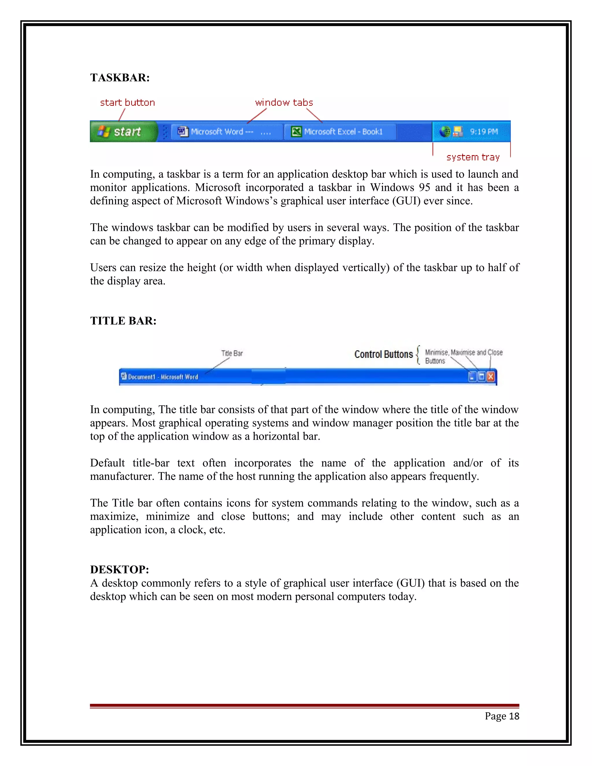
TASKBAR:
In computing, a taskbar is a term for an application desktop bar which is used to launch and
monitor applications. Microsoft incorporated a taskbar in Windows 95 and it has been a
defining aspect of Microsoft Windows’s graphical user interface (GUI) ever since.
The windows taskbar can be modified by users in several ways. The position of the taskbar
can be changed to appear on any edge of the primary display.
Users can resize the height (or width when displayed vertically) of the taskbar up to half of
the display area.
TITLE BAR:
In computing, The title bar consists of that part of the window where the title of the window
appears. Most graphical operating systems and window manager position the title bar at the
top of the application window as a horizontal bar.
Default title-bar text often incorporates the name of the application and/or of its
manufacturer. The name of the host running the application also appears frequently.
The Title bar often contains icons for system commands relating to the window, such as a
maximize, minimize and close buttons; and may include other content such as an
application icon, a clock, etc.
DESKTOP:
A desktop commonly refers to a style of graphical user interface (GUI) that is based on the
desktop which can be seen on most modern personal computers today.
Page 18

· These graphical user interfaces are designed to assist the user in easily accessing and
configuring (or modifying) the most important (or frequently accessed) specific OS packed
features.
· A desktop environment typically consists of icons, windows, toolbars, folders, wallpapers.
· Software which provides a desktop environment might also provide drag and drop
functionality and other features which make more complete.
· Today, most popular personal computers come pre-installed with an OS that provides a
desktop environment. Traditionally these computers have used Microsoft Windows and to a
lesser extent Mac OS whose desktop environments are relatively unalterable.
· The most common desktop environment on personal computers is the one provided by
Microsoft Windows; another common environment is the one provided by Apple Mac OS.
NETWORK NEIGHBORHOOD:
If your PC is connected to a network, the network neighborhood folder displays all
computers in your network. To open the network neighborhood folder, double-click the
network neighborhood icon on your desktop or in window explorer. Then windows display
the network neighborhood window. This network neighborhood displays a list of all
computers that are connected to the network.
On double clicking icon, window will display the resources of the computer which you have
access right to. Therefore, you may not be able to access all folders on all hard disks on a
particular computer. Moreover, depending on the different types of rights (such as read,
write, delete etc,) you may be able to open , edit or delete files on the folder of other
computer on the network.
If you are connected on a network and you have rights to save files on other computer, you
can specify the other computer’s folder as the path.
Page 19

WHAT IS FILE?
File is a collection of text or data stored on a storage device, such as a floppy disk or hard
disk. You can store different types of documents in conventional file, the file that stores
letters, memos, documents, etc is known as document or text file. The file that stores
database information, such as an address list or sales information for a period is called
database file. A file that contains instructions written in a programming language is called a
program file.
Control Panel, recycle Bin and Page Orientation
 Control Panel
The control panel is used to control the computer system. For example, you can control the
behaviour of your mouse, keyboard, display, modem, printers, etc. Let us have a look at the
control Panel.
® Open the start menu by clicking the start button on the taskbar.
® Choose the settings command from the start menu. (you can choose a command
either by clicking / moving the mouse on the command or by using the keyboard)
® Windows displays a submenu of commands for settings. This submenu contains
‘Control Panel’ besides other commands.
® Choose the control panel command.
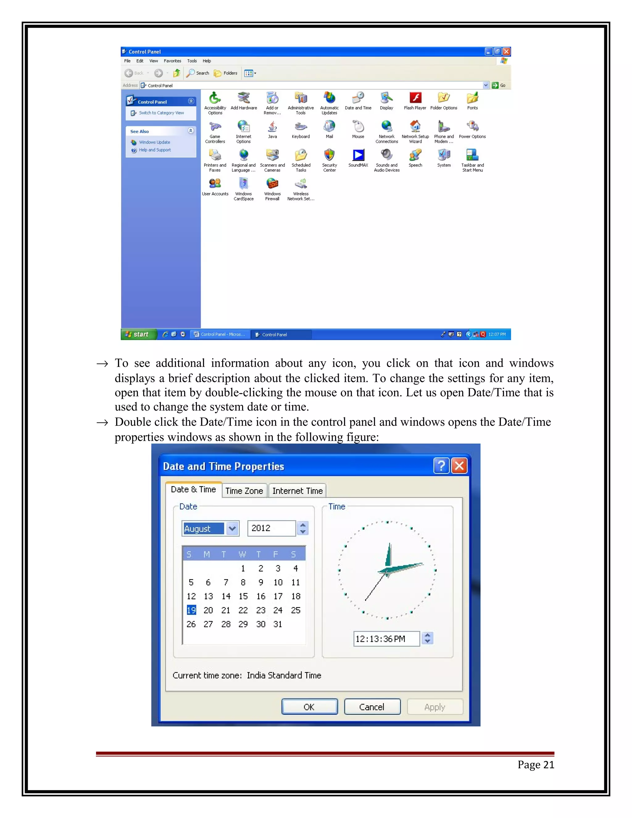
® Windows displays the control panel window that contains several icons as shown in
the following figure:
Page 20

® To see additional information about any icon, you click on that icon and windows
displays a brief description about the clicked item. To change the settings for any item,
open that item by double-clicking the mouse on that icon. Let us open Date/Time that is
used to change the system date or time.
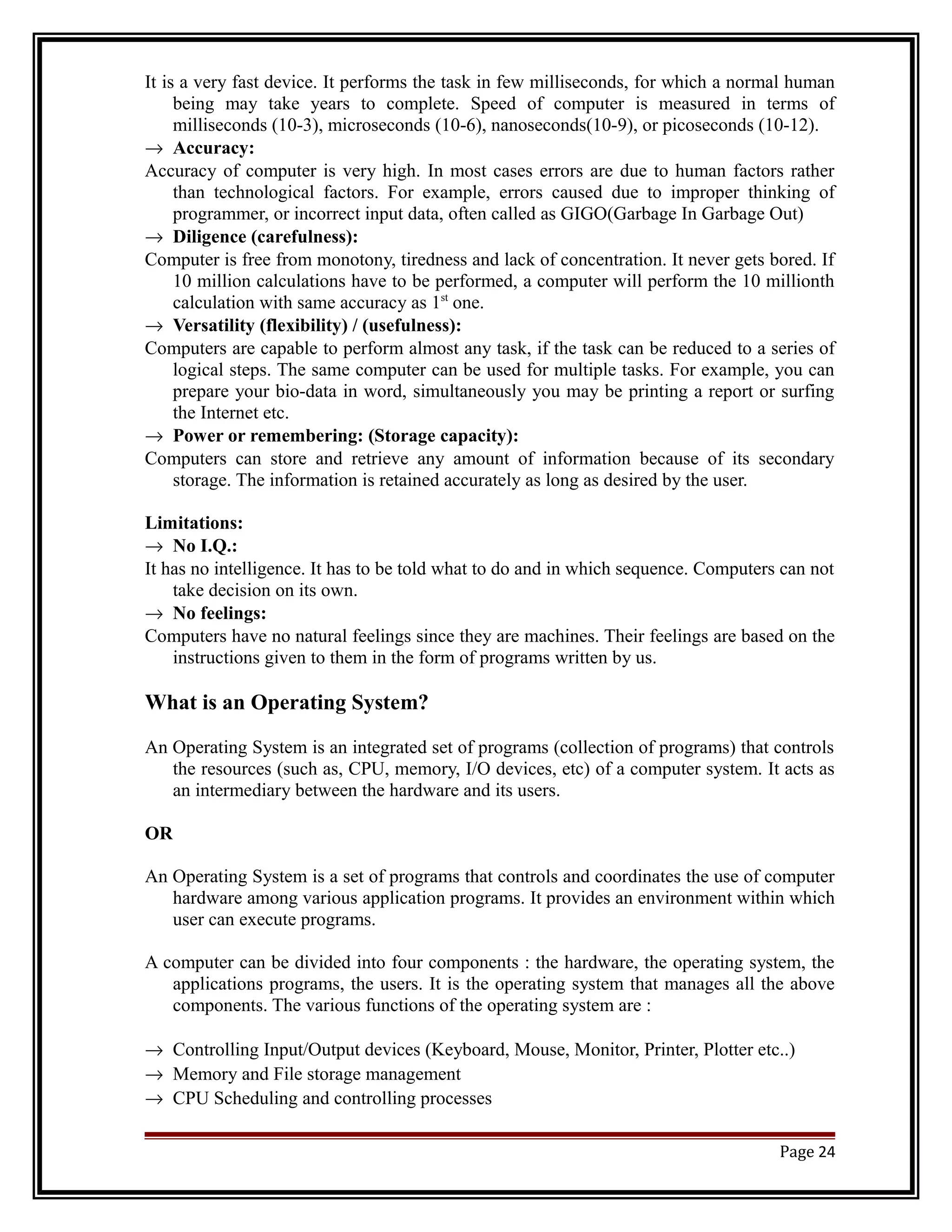
® Double click the Date/Time icon in the control panel and windows opens the Date/Time
properties windows as shown in the following figure:
Page 21

® After adjusting the date and / or time, click the OK button to ask Windows to use the
new settings and close the Date/Time Properties window. However, if you do not
want to use the new date/time settings, click the Cancel button or close button in
the title bar.
RECYCLE BIN
Microsoft introduced the recycle bin in the windows 95 Operating System. The Recycle Bin
keeps files that have been deleted, whether accidentally or intentionally. Users can review
the contents of the Recycle Bin before deleting the items permanently. The Recycle Bin
holds data that not only lists deleted files, but also the date, time and the path of those files.
The Recycle Bin is opened like ordinary Windows Explorer folder and the files are viewed
similarly. Deleted files may be removed from the Recycle Bin by restoring them with a
command, or by deleting them permanently.
In Recycle Bin window, you can restore (i.e. undelete) all items back to their original
locations by clicking restore all. If you want to restore selected items, select the require
items and then choose the restore command from the file menu or from the right click
menu. If you want to get details about any item in the Recycle Bin, select the item and the
recycle bin displays it in window.
The number of items the recycle bin can hold is limited by the hard disk space allocated to it
by windows. Therefore, you should periodically empty the recycle bin by deleting those
items from the recycle bin that you no more want to restore. For doing this, select the items
and use the delete command from the file or the right click menu. to remove all items from
the recycle bin, use the empty recycle bin command from file menu.
The recycle bin’s icon indicates whether there are items in the Recycle Bin. If there are no
files or folders in the Recycle Bin, then the icon resembles an empty wastepaper basket.
Othwerwise if there are files and/or folders the icon resembles a full wastepaper basket. If
your recycle bin window is empty, it indicates that currently there are no deleted items.
The recycle bin can be accessed via the desktop or Windows Explorer. Files are moved to
recycle bin in a number of ways.
® By right clicking on a file and selecting delete from the menu.
® Selecting a file and pressing delete key.
® By dragging and dropping a file into the recycle bin icon.
The recycle bin only stores files deleted from hard drives, not from removable media, such
as memory cards, floppy disks, pendrives. It also doesn’t stores files deleted from network
drives.
PAGE SETUP
Question: What is page orientation?
Ans: When you create a new document , word picks up a paper size, which is usually the Letter
Size (8.5” wide x 11” long), or A4 Size. Let us check up the paper size that is in use for the
current document.
Page 22

® Click the paper size tab boxes in the page setup dialog box. This tab is located on the
right side on the Margins tab (See in the figure)
· Word displays information about paper size in the page setup dialog box as shown in
the figure.
· Click the drop down arrow on the right side of the paper size box and word displays
a list of standard paper sizes.
· If you are using a paper size that is there in the list, you can select it from the list.
· Word allows you to change the orientation of the page.
· The default orientation is portrait.
· If you change the orientation to Landscape, word swaps the width and height of the
page.
· That is in the landscape orientation, the letter size page becomes 11” wide and 8.5”
high.
· It increases the width of the page but reduces the height.
What is a Computer?
Computer is an electronic device, which can automatically accept and store input data,
process them and produce output results according to the instructions given by the
programmer or user.
Explain the characteristics and Limitations of a computer.
Characteristics:
® Speed:
Page 23

It is a very fast device. It performs the task in few milliseconds, for which a normal human
being may take years to complete. Speed of computer is measured in terms of
milliseconds (10-3), microseconds (10-6), nanoseconds(10-9), or picoseconds (10-12).
® Accuracy:
Accuracy of computer is very high. In most cases errors are due to human factors rather
than technological factors. For example, errors caused due to improper thinking of
programmer, or incorrect input data, often called as GIGO(Garbage In Garbage Out)
® Diligence (carefulness):
Computer is free from monotony, tiredness and lack of concentration. It never gets bored. If
10 million calculations have to be performed, a computer will perform the 10 millionth
calculation with same accuracy as 1st one.
® Versatility (flexibility) / (usefulness):
Computers are capable to perform almost any task, if the task can be reduced to a series of
logical steps. The same computer can be used for multiple tasks. For example, you can
prepare your bio-data in word, simultaneously you may be printing a report or surfing
the Internet etc.
® Power or remembering: (Storage capacity):
Computers can store and retrieve any amount of information because of its secondary
storage. The information is retained accurately as long as desired by the user.
Limitations:
® No I.Q.:
It has no intelligence. It has to be told what to do and in which sequence. Computers can not
take decision on its own.
® No feelings:
Computers have no natural feelings since they are machines. Their feelings are based on the
instructions given to them in the form of programs written by us.
What is an Operating System?
An Operating System is an integrated set of programs (collection of programs) that controls
the resources (such as, CPU, memory, I/O devices, etc) of a computer system. It acts as
an intermediary between the hardware and its users.
OR
An Operating System is a set of programs that controls and coordinates the use of computer
hardware among various application programs. It provides an environment within which
user can execute programs.
A computer can be divided into four components : the hardware, the operating system, the
applications programs, the users. It is the operating system that manages all the above
components. The various functions of the operating system are :
® Controlling Input/Output devices (Keyboard, Mouse, Monitor, Printer, Plotter etc..)
® Memory and File storage management
® CPU Scheduling and controlling processes
Page 24

® Loading, initiating, executing and supervising user applications programs
® Handling errors and restarting
® Providing command interface between user and computer system
Examples of Operating system are : UNIX (Solaris, IRIX, HPUnix, Linux, DEC Unix)
Microsoft Disk Operating System (MS-DOS), WIN95/98, WIN NT, OS/2 etc.
(http://www.imtech.res.in/raghava/slides/prephd/doslec.htm)
Types of Operating Systems
Within the broad family of operating systems, there are generally four types, categorized
based on the types of computers they control and the sort of applications they support.
The categories are:
· Real-time operating system (RTOS) - Real-time operating systems are used to control
machinery, scientific instruments and industrial systems. An RTOS typically has very
little user-interface capability, and no end-user utilities, since the system will be a
"sealed box" when delivered for use. A very important part of an RTOS is managing the
resources of the computer so that a particular operation executes in precisely the same
amount of time, every time it occurs. In a complex machine, having a part move more
quickly just because system resources are available may be just as catastrophic as
having it not move at all because the system is busy.
· Single-user, single task - As the name implies, this operating system is designed to
manage the computer so that one user can effectively do one thing at a time. The Palm
OS for Palm handheld computers is a good example of a modern single-user, single-task
operating system.
· Single-user, multi-tasking - This is the type of operating system most people use on
their desktop and laptop computers today. Microsoft's Windows and Apple's MacOS
platforms are both examples of operating systems that will let a single user have several
programs in operation at the same time. For example, it's entirely possible for a
Windows user to be writing a note in a word processor while downloading a file from
the Internet while printing the text of an e-mail message.
· Multi-user - A multi-user operating system allows many different users to take
advantage of the computer's resources simultaneously. The operating system must make
sure that the requirements of the various users are balanced, and that each of the
programs they are using has sufficient and separate resources so that a problem with one
user doesn't affect the entire community of users. Unix, VMS and mainframe operating
systems, such as MVS, are examples of multi-user operating systems.
Main Functions of an Operating System?
The main functions of an Operating System is as follows:
(1)Process Management:
Page 25

The process management module of an operating system takes care of the creation and
deletion of processes, scheduling of various system resources to the different processes
requesting them and providing mechanisms for synchronization and communication
among processes.
(2) Memory management:
The memory management module of an OS takes care of the allocation and deallocation
of memory space to the various programs in need of this resources.
(3) File management:
The file management module of an OS takes care of file-related activities such as
organization, storing, retrieval, naming, sharing and protection of files.
(4) Security:
The security module of an OS protects the resources and information of a computer system
against destruction and unauthorized access.
(5) Command interpretation:
The command interpretation module of an OS takes care of interpreting user commands,
and directing the system resources to handle the requests. With this mode of interaction
with the system, the user is usually not too concerned with the hardware details of the
system.
Main Features of an Operating System?
Different operating systems have differing features, though they all have the primary function
of
controlling the software and programs running on a computer or other device.
http://www.teach-ict.
com/as_as_computing/ocr/H447/F453/3_3_1/features_of_os/miniweb/pg11.htm
You now have read about the various kinds of operating systems that are part of computers
ranging from a humble mobile phone to a mighty supercomputer taking up an entire
building.
But they share some common features, some of which are more important than others
depending
on the type of operating system Scheduling The task of handling how active processes are
making efficient use of the CPU processing cycles is called scheduling. There are many ways of
doing this, which is covered in another mini-website.
Memory Management
The operating system has to make sure that applications are able to run in the amount of
memory
available and that they do not interfere with one another. There is a separate mini-website on
this
topic.
Page 26

Allocation of resources
The operating system will provide a working area for each user. This includes
Disk space quota for their files ( especially on shared network drives)
A personal GUI set up for each user (multi-user operating systems)
Perhaps how many processing cycles they are allowed to use (especially on mainframe)
How much printer output they are allowed (networked and mainframe)
How high a priority they can assign to a job (mainframe)
Keeping track of usage
The cost of using large computers is shared amongst the users. So the operating system will
have
an accounting / tracking system in place that :
Counts the processing cycles used per user
Print out jobs completed
Batch jobs completed
Time spent logged in
Other resources used
And so on. A regular bill is then sent to the user account providing an itemized (detailed)
charge.
Data and User security
Each user has to be authenticated with an username and password (network and multi-user
operating system).
Their data and files will be kept private from other users, unless they choose to make some
shareable with others. The operating system will only allow administrators ('super
users') to change parts of the operating system and install applications.
Providing system services such as print spooling
Printing out is a time consuming process, so it makes sense to allow users to hand-off a print
job
to the operating system so they can get on with other things. This is called 'print spooling' and is
common on multi-user and networked operating systems.
Managing input / output
Data and applications are stored on secondary storage devices such as hard disks, optical drives,
magnetic tape when not in use. The operating system has a file management system that allows
the user to organize their files, to move, delete and copy files as they wish.
Specialized input devices such as graphics tablets and scanners are also handled by the
operating system.
Page 27

Handling Network communication
Data packets traveling to and from the connected computers on the network are handled by the
operating system.
When an user drags a file from their hard disk to a shared networked drive, they do not care
how
it happens - the operating system takes care of all the details
EXPLAIN BLOCK DIAGRAM OF A COMPUTER:
INPUT UNIT:
PROCESS
A.L.U.
C.U.
Registers
Main
Memory
Data and instructions must be entered into the computer system before any computation can
be performed on the supplied data. The input unit performs this task. It links the external
environment with computer system. Functions performed by an input unit are as
follows:
® Accepts or reads the list of instructions and data from the outside world.
® Converts these instructions and data in the computer acceptable form (binary codes).
This transformation is done by units called input interfaces.
® Supplies the converted instructions and data to the computer system for further
processing.
® Input unit consists of one or more input devices like keyboard, mouse, scanner etc.
OUTPUT UNIT:
Page 28
INPUT OUTPUT
C.P.U.
Secondary Memory

The job of output unit is reverse of input unit. It links the computer system with external
environment. Tasks performed by output units are as follows:
® Accepts results produced by the computer, which are in the coded form and hence
cannot be easily understood by us.
® It converts coded results to human acceptable (readable) form.
® It supplies the converted results to outside world.
® Output unit consists of one or more output devices like printer, monitor, speaker etc.
C.P.U.: (Central Processing Unit):
The C.P.U. is the heart of the computer. It comprises of :
C.U. (control unit):
Control unit is mainly responsible for controlling all the unit of operations in the computers.
It obtains instructions from the program stored in main memory; interpret the
instructions; and issues signals that cause other units of the system to execute them.
A.L.U. (Arithmetic Logical Unit):
ALU is the place where the actual execution of the instruction takes place. All the
calculations and comparisons are performed in ALU. Almost all ALUs are designed to
perform the four basic operations – add, subtract, multiply, divide and logic operations
or comparison such as less than (<) or greater than (>).
REGISTERS:
Registers are small high speed memory used to store temporary results and certain control
information. Each register has a certain size and function. Registers can be read and
written at high speed since they are internal to C.P.U.
STORAGE UNIT:
This unit holds all the data to be processed and instructions required for processing,
intermediate results of processing, and final results of processing before these results are
released to an output unit. Two major types of storages are:
(1) Primary Storage / Main Memory / Temporary Storage:
It holds the part of instructions and data of currently running program, intermediate results
of processing and final result of processing unit until it is transferred to some
appropriate space. The CPU can access the content of RAM directly. It has limited
storage capacity. It is expensive. It is volatile i.e. it losses content if power supply is cut
off. It is faster than secondary storage, e.g. RAM, ROM, Cache etc.
(2) Secondary Storage / Auxiliary Storage / Permanent Storage:
It is used to store large amount of instructions and data. C.P.U. is not capable of directly
accessing data and programs residing on the secondary storage. So, if data need to be
processed or instruction needs to be executed, it must be transferred to primary storage.
It is cheaper than primary storage. It is non volatile i.e. it retains content even though
power supply is cut off. It is slower than primary storage. e.g. Hard Disk, CD, DVD,
Floppy Disk etc.
Software:
The set of computer programs, procedures and associated documents (flowcharts, user
manuals etc,), which describes the programs and how they are to be used, whose
objective is to enhance the capabilities of H/W.
Page 29

Software
System Software Application Software
System
Management
Programs
System
Support
Programs
System
Development
Programs
General
Purpose
Application
Software
Special
Purpose
Application
Software
A Software can be divided into two major categories
System Software
System Software is a set of one or more programs, designed to control the operation and
extend the processing capability of a computer system. System software makes the
operation of computer more effective and efficient. Actually, system software is any
computer software which manages and controls computer hardware so that application
software can perform a task.
In general system software performs following functions:
® System software performs tasks like transferring data from memory to disk, or rendering
(Representing) text onto a display device.
® Specific kinds of system software include loading programs, operating systems, device
drivers, programming tools, compilers, assemblers, linkers, and utility software.
® It supports development and execution of other application software.
® It monitors the effective use of various hardware resources, such as CPU, Memory,
peripherals etc,.
® It communicates with and controls the operation of peripherals devices, such as printer,
disk, tape, etc.
® E.g:. Operating systems, such as Microsoft Windows, Mac OS X or Linux, are well-known
examples of system software.
System software mainly includes 3 different types of programs:
(1) System Management Programs:
They manage Hardware and Software of computer system.
e.g. Operating Systems
(2) System Support Programs:
They provide support services to users. e.g. Utility Programs.
Page 30

(3)System development Programs:
It helps developers in designing and building system. e.g.
Language translator (compiler, interpreter etc.)
Application Software
Application Software is a set of one or more programs, design to solve specific problem, or to do a
specific task. This application software can be classified into two categories:
(1) General Purpose Application Software:
General purpose application software provides certain generalized facilities. They are
generally pre-written. e.g. Word Processing (MS-Word), Spreadsheet Application (MS
Excel), Database Application packages etc.
(2) Special Purpose Application Software:
Application programs specific to certain area / users for their specific requirement are
called Special purpose application software. They are custom build. e.g. Inventory
management, Payroll System etc.
Difference between System Software and Application Software
System Software Application Software
1 It is a set of one or more
programs, designed to
control and co-ordinate
the operations of a
computer system.
1 It is a set of one or more programs,
designed to solve specific
problem or to do a specific task.
2 It is machine oriented 2 It is user oriented.
3 It can execute without help
of other software
3 It generally takes the help of system
software to execute.
4 e.g. operating system,
utility software etc.
4 e.g. Student Management system,
Payroll System etc.
 Levels of programming languages:
OR
 What are High level and Low level language?
Ans:
Programs are classified under three main categories. They are
1. Machine level
2. Assembly level
3. High Level
1. Machine level language (MLL):
It is 1st Generation language. It is a language of 1’s and 0’s. This 1’s and 0’s are referred as
binary code or machine code. Computer can understand this binary code directly or easily.
Advantages:
Page 31

® Faster execution
® Computer understands easily
Disadvantages:
® It is machine dependant and not portable
® Size is larger
® Difficult to code
® Debugging (Error solving) is very difficult
2. Assembly level language (ALL):
It is an intermediate language. It is written using mnemonics and 1’s and 0’s. This is the 2 nd
generation language. It is also known as low level language. Since computer cannot understand
it directly it needs to be translated into machine level language. It requires a program called
assembler for converting assembly code to machine code.
Advantages:
® It is convenient than machine language.
® User friendly as user can code it easily compared to MLL.
® Size of the program is reduced as compared machine level language.
Disadvantages:
® It is machine dependant and so not portable
® Takes more execution time than machine level language.
® Computer cannot understand directly it requires translator.
3. High Level Languages (HLL):
Programs are written in English. The Programs cannot be executed directly. It needs to be
converted to machine level language for execution. It requires a translator called Compiler or
Interpreter for converting HLL to MLL. Programs are written in BASIC, COBOL, FORTRAN,
PASCAL, C etc. These programs are also called Procedure Oriented Languages. These languages
are also called 3rd Generation languages. Programmer needs to specify complete instructions in
order to perform a task.
Advantages:
® Portable i.e. Machine Independent
® User can understand easily
® User can write programs easily
Disadvantages:
® Execution time is more
® Computer cannot understand directly.
4. Fourth Generation Language:
These are Non Procedure Oriented Languages. It requires outline not detailed instructions to
perform a task as compared to HLL. It is commonly referred to as 4GL. They are used to work
with files and databases. They are also called as query languages.
Page 32

Que: Difference between primary memory and Secondary memory.
Ans:
Primary Memory Secondary Memory
1 It stores programs and data
which are currently
needed by the CPU.
1 The information which is not
currently being processed
resides in secondary memory.
2 Semiconductor memory is
used as primary memory
2 Magnetic or Optical memory is
used as Secondary memory
3 It is faster compared to
secondary memory
3 It is slower compared to Primary
memory
4 It has higher cost per bit of
storage
4 It has lower cost per bit of storage.
5 It has low storage capacity 5 It has much large storage capacity
than primary memory.
6 The CPU communicates
directly with main
memory,
6 The CPU does not communicates
directly with secondary
memory.
7 It is usually contained on the
mother board.
7 The secondary memory is the
external memory.
8 E.G. RAM, ROM, etc,. 8 E.G. Hard Disk, CDs, etc,.
Page 33

MS-Office is a product of Microsoft Company. Ms office is a collection of Application
Software. Mainly three Software are there:
(1) Microsoft Word (2) Microsoft Excel (3) Microsoft Power
Point
MS-WORD Microsoft Word is a Word Processor Software. (શબદ પર પિકયા કરનાર સોફટવેર). It is a Window bases
Application software. Into which user can do different types of work, for example, document
typing, letter typing, bio-data and application making etc.
Steps for Start: START  All Programs  Microsoft Office  Microsoft Word
Screen Introduction of Word:
http://www.functionx.com/word/Lesson01.htm
Page 34

On the most left side of the title bar, there is an icon that represents the application. That
application icon also represents menu used to perform many operations related to
Microsoft Word as an application.
To use the system menu on the application icon, click the small icon
A menu appears. From the system menu, click Restore
To maximize the application again, click the icon again, and click Maximize from the menu.
On the right side of the icon, there are two groups of words. When Microsoft Word starts, it
creates an empty document called Document1. It is called default name of Microsoft Word.
You can then type your text. If at one time you find that you need another document, you
can initiate a second one. In that case, you would have Document2. Eventually you can
add more documents. We will come back to that feature. DocumentX represents the name
of the file you are working on. If you save your document under an appropriate name, the
new name would display in that area and Document1 or DocumentX would disappear.
On the right side of Document is the name of the application. Microsoft Word would like
you to know that it is the running application.
On the right side of the application’s name, there is a long empty bar; this is the main area
of the title. As empty as it looks, this area can be used to perform many actions because it
has a menu of its own.
To experiment with the title bar, double-click it. The window is restored
The File extension for the Microsoft Word file is .doc (in MS word 2003) and .docx (in MS
word 2007).
 F ile Menu: (alt + F)
® N ew (ctrl + N): With the help of this option you can create a new file in your word
document.
STEPS:
(1) Click on File Menu
(2) Click on New option
(3) Select blank document
(4) Click on OK button.
® O pen (ctrl + O): With the help of this option you can open a previously created file in
your word document.
STEPS:
(1) Click on File Menu
(2) Click on Open option
(3) In Look in: box, select a folder where your file is located.
(4) In File name: box, give a file name to open.
(5) Click on Open button.
Page 35

® Save (ctrl + S): With the help of this option you can save a file.
STEPS:
(1) Click on file menu.
(2) Click on Save option.
(3) In Save in: box, select a folder, where you want to save your word file.
(4) In File name: box, give a proper file name to save your file.
(5) Click on Save button.
® Save As: With the help of this option you can save a file with different / another name.
it
means you can create a copy of a file.
STEPS:
(2) Select Save As option
(3) In Save in:, box, select a folder, where you want to save your word file.
(4) In File name: box, give a proper file name to save your file.
(5) Click on save button.
® Close: with the help of this option you can close a word file.
STEPS:
(1) Click on File menu.
(2) Select close option.
® P rint (ctrl + P): With the help of this option you can take a print of your file.
STEPS:
(2) Select print option.
® Print Preview: With the help of this option you can view a file before taking a print.
STEPS:
(2) Select print preview option.
® Page Setup: With the help of this option you can set your page. It means you can set a
page margin as well as gutter (a Space for biding). You also set orientation
(Portrait, Landscape).
STEPS:
(2) Click on page setup option.
(3) Set Left margin, Right margin, Top margin , Bottom margin and Gutter
for the page.
(4) If you want to set orientation, then click on PAGE SIZE button / tab.
(5) Select one of the two orientations.
® Exit: With the help of this option you can close a word or exit from the word.
STEPS:
(2) Select Exit option.
Steps for save a file with Password:
(1) Click on File Menu.
Page 36

(2) Click on Save As option.
(3) Click on Tools.
(4) Click on General Option / Security Option.
(5) In Password to open: box, give a password
(6) Click on OK
(7) In Reenter Password to open: box, reenter the previously given
password.
(8) Click on OK button
(9) In File name:, box, give a proper file name
(10) Click on save button.
 E dit Menu (alt + E):
® Undo (ctrl + Z): With the help of this option you can cancel your last command effect. It
means it allow us to reverse the last action we have performed. Undo
is
one Step backward from the Current Step.
STEPS:
(1) Click on Edit menu.
(2) Select Undo Option.
® Redo (ctrl + Y): With the help of this option you can cancel your undo effect. It
means it allow us to redo an action that we undid by mistake. Redo is
one Step forward from the Current Step.
STEPS:
(2) Select Redo option.
® Copy (ctrl + C) & Paste (Ctrl + V): With the help of this option you can copy a text and
picture.
STEPS:
(1) Select a Text or Picture you want to copy
(3) Select a copy option.
(4) Set your cursor position
(5) Click on edit menu again
(6) Select paste option.
® Cut (ctrl + X) & Paste (Ctrl + V): With the help of this option you can move a text and
picture from one location to another location. (One
place to another place)
STEPS:
(1) Select a Text or Picture you want to cut / move
(3) Select a cut option.
(4) Set your cursor position.
(5) Click on edit menu again.
(6) Select paste option.
® Clear (del): With the help of this option you can delete a selected text and picture.
STEPS:
Page 37

(1) Select a Text or Picture you want to delete
(3) Select clear option.
® Select All (Ctrl + A): With the help of this option you can select a whole document.
STEPS:
(2) Click on Select all option.
® Find (Ctrl + F): With the help of this option you can find a text in your word file /
document.
STEPS:
(2) Click on find option.
(3) In Find what: box, type a word or a text, which you want to find.
(4) Click on “Find Next” button.
® Replace (Ctrl + H): With the help of this option you can replace a text(word) by another
text (word).
STEPS:
(2) Click on replace option.
(3) In Find what: box, type a word or a text which you want to replace.
(4) In replace with: box, Type a word or a text by which you want to
replace a previous word or a text.
(5) Click on Replace button.
® Go to (Ctrl + G): With the help of this option you can jump to the particular line number
or particular page in your word document.
STEPS:
(2) Click on Go to option.
(3) In Go to What: box, give a line number or page number on to which you
want to jump.
(4) In Enter number: box, give a number to jump. (If you want to jump 4
line forward from the current line then write +4, or if you want to jump
4 line back ward from the current line then write -4 in the box.).
(5) Click on Go to button.
 V iew Menu (alt + V):
® In Ms Word, there are mainly 4 types of viws: (1) Normal (2) Print Layout (3) Web
Layout (4) Outline
(1) Normal: With the help of this option you can view your document or a file in normal
view. In this type of view margin, header, footer and page border does not displayed.
STEP:
(1) Click on View menu.
(2) Select normal option.
(2) Print Layout: With the help of this option you can view your document or a file in Print
Layout view. In this type of view margin, header, footer and page border has been
displayed.
Page 38

STEPS:
(2) Select print layout option.
(3) Web Layout: With the help of this option you can view your document or a file in
HTML or web layout view.
STEPS:
(2) Select Web layout option.
(4) Outline: With the help of this option you can view your document or a file in outline
view.
STEPS:
(2) Select outline option.
® Tool Bar: with the help of this option of view menu you can ON or OFF a toolbar.
STEPS:
(1) Click on View Menu
(2) Select toolbar option
(3) Select toolbar which you want to ON or OFF.
® Ruler: With the help of this option you can ON or OFF a ruler.
STEPS:
(1) Click on view menu
(2) Select Ruler option for ON or OFF.
® Header and Footer: With the help of this option you can insert a header and a footer into
your document.
STEPS:
(1) Click on View menu
(2) Select Header and Footer option
(3) In Header box, Give a header
(4) In footer box, give a footer
(5) Click on close
® Full Screen: With the help of this option you can view a document file in a full screen
mode. In full screen mode Menu bar, Tool bar and a task bar does not
displayed.
STEPS:
(2) Select full screen option
(3) For close a full screen click on close full screen button.
® Zoom: With the help of this option you can view your document in bigger size than the
normal size.
STEPS:
(2) Select zoom option
(3) In Zoom to box, give a percentage to view
 I nsert Menu (alt + I):
Page 39

® Page Break (ctrl + Enter): With the help of this option you can insert a page break into
your document.
STEPS:
(1) Click on Insert Menu
(2) Select Break Option
(3) Select Page Break from it
(4) Click on OK Button.
® Page No: With the help of this option you can insert a page no into your document.
STEPS:
(2) Select Page No option
(3) Select your cursor position
(4) Select Alignment
® Date & Time: With the help of this option you can insert date and time into your
document.
STEPS:
(1) Click on Inset menu
(2) Select Date & Time Option
(3) Select any one format of Date & Time.
® Picture  Clip Art: With the help of this option you can insert a Clip Art in your
document.
STEPS:
(2) Select picture option
(3) Click on clipart option from it
(4) Select any one category of a picture
(5) Click on Insert Clip button
(6) Close Clipart dialog box.
® Picture  Word Art: With the help of this option you can insert a Word Art in your
document.
STEPS:
(2) Select Picture option
(3) Select WordArt option
(4) Select any one WordArt Style
(6) Write any text.
® Picture  Auto Shape : With the help of this option you can insert a Auto Shape in
your
Document.
STEPS:
(2) Select Picture Option
(3) Select Auto Shape option
Page 40

(4) Select any one category of Auto Shape
(5) Select any shape from it
(6) Drag and drop a mouse.
® Text Box: With the help of this option you can insert a Text Box in your
Document.
STEPS:
(2) Select Text Box Option
(3) Drag and Drop the mouse to set that Text Box in your document.
(4) After Writing the text into the textbox, click outside of the Text Box.
® Symbol : With the help of this option you can insert a special Symbols into your
document which are not available onto your keyboard.
STEPS:
(2) Select Symbol option
(3) Select any one symbol from it
(4) Click on Insert Button
(5) Click on close button.
® Auto Text: With the help of this option you can insert an auto text into your document.
STEPS:
(1) Click on Insert menu
(2) Select Auto text option
(3) Select Auto text option in another text box also.
(4) Enter a text which you want to add into your document.
(5) Click on Insert button.
STEPS FOR INSERTING A TEXT IN AN AUTO TEXT GROUP:
(2) Select Auto text option
(3) Select Auto text option in another text box also.
(4) Enter Auto Text Entry Here  Add a text which you want to add in auto
text group
(5) Click on ADD button
 Format Menu (alt + O):
® Font : With the help of this option you can format a font, for example, you can
change font type, font colour, font style, underline style and colour and
also can apply effect to the text.
STEPS:
(1) Select a text which you want to format
(2) Click on Format Menu
(3) Click on Font option
(4) Select Font, Font size , font style etc.
(5) If you want to put underline then select underline style and colour and
also choose effect for the text
STEPS FOR SUPERSCRIPT (A2 + B2) AND SUBSCRIPT (H2O):
Page 41

(1) Write A2 + B2 first
(2) Select 2 from it.
(3) Click on Font option
(4) Select Super script or Subscript effect as you want
® Bullets and Numbering: With the help of this option you can insert bullets and
numbering
into your document
STEPS:
(1) Click on Format menu
(2) Select bullets and numbering option from it
(3) Select bullets Or Number option from it.
(4) Select any one style of a bullets
® Border and Shading: With the help of this option you can insert border and shading on
selected text as well as also apply shading and border to the
document page also.
STEPS:
(1) Select a text on which you want to apply shading or border’
(2) Click on format menu
(3) Click on border and shading option
(4) Select any one style of a border
(5) Select any one border colour
® Paragraph: With the help of this option you can set an format a paragraph into your
document. For example you can set alignment, and space between two lines
as
well as character etc.
STEPS:
(1) Select a paragraph which you want to format
(2) Click on format menu
(3) Click on paragraph option from it
(4) In Alignment box, Set your paragraph alignment. Indent your paragraph
left or right according to your requirement. Also set spacing between two
lines.
(5) Close Paragraph dialog box.
® Columns: With the help of this option you can divide a document into more than one
part or a column.
STEPS:
(2) Select column option
(3) Select any column style from it.
® Drop Cap: With the help of this option you can apply a Drop Cap effect on a character.
STEPS:
(1) Select a Character on which you want to apply a Drop Cap Effect.
(3) Select Drop Cap option
Page 42

(4) Select any one effect from it
Drop Cap: A drop cap is a single letter made large than the others in a paragraph. It is
the first letter in a section and, as a drop cap, is in a separate text box. It is used to
draw the eye to the beginning of the section. Drop caps are often seen at the
beginning of novels.
® Change Case: With the help of this option you can change a case of a text.
STEPS:
(1) Select a text
(3) Select Change Case option from it
(4) Select any one case from it
NOTE: Refer Big Question of Change Case and steps
® Back Ground: With the help of this option you can apply or insert a background into
your
document.
STEPS:
(1) Click on Format Menu.
(2) Select Background Option from it.
(3) Click on Fill Effect
(4) Click on Present
(5) Click on Present Colour
(6) Select any one colour from the present colour
(7) Select any one shading style
 Table Menu (alt + A):
Table: Combination of Rows and Columns is known as table.
Rows: In Table, Horizontal Lines are called as Rows.
Columns: In table, Vertical lines are called as Columns.
Cell: Intersection of Rows and Columns are known as cell.
® Table  Insert  Table: With the help of this option you can insert a table into your
document.
STEPS:
(1) Click on table Menu
(2) Click on Insert option
(3) Select table sub-option from it
(4) In Number of Column box, give a number of columns as you want.
(5) In number of rows box, give a number of rows as you want.
® Table  Insert  Cell: with the help of this option you can insert a cell into table.
Page 43

STEPS:
(1) Set a position of a cursor in a table
(2) Click on table Menu
(3) Select Insert option
(4) Click on Cell sub-option from it
® Table  Insert  Column: With the help of this option you can insert a column into
your
table.
STEPS:
(1) Set a position of a cursor in a table
(2) Click on Table menu
(3) Click on Insert option
(4) Choose columns to the left or right according to requirement
® Table  Insert  Row: With the help of this option you can insert a rows into your
table.
STEPS:
(1) Set a cursor position in the table
(2) Click on table menu
(3) Select insert option
(4) Choose rows above or below according to requirement
® Table  Delete  cell: With the help of this option you can delete a particular selected
cell from your table.
STEPS:
(1) Selecta cell which you want to delete.
(3) Select delete option
(4) Select cell sub-option from it
(5) Select an option (up, down, entire row) as according to requirement
® Table  Delete  column: With the help of this option you can delete a particular
selected column from your table.
STEPS:
(1) Select a column which you want to delete
(2) Click on Table Menu
(3) Click on Column option
® Table  Delete  Row: With the help of this option you can delete a particular
selected
row from your table.
STEPS:
(1) Select a row which you want to delete
(3) Select a delete option
(4) Select a row sub-option from it.
® Table  Delete  table: With the help of this option you can delete an entire table.
Page 44

STEPS:
(1) Set your cursor position anywhere in the table
(3) Select Delete option
(4) Click on Table sub-option from it.
® Table  Merge cell: With the help of this option you can merge two or more than two
cells.
STEPS:
(1) Select a cells or a rows or a columns which you want to merge
(3) Select Merge option from it
® Table  Split cell: With the help of this option you can split or divide a cell into two or
more than two parts.
STEPS:
(1) Select a cell which you want to split
(3) Select Split cell option
(4) In Number of column box, give a number into which you want to split a
cell
(5) In Number of rows box, give a number into which you want to split a
cell
® Table  Split table: With the help of this option you can split an entire Table.
STEPS:
(1) Set a cursor position from which you want to split your table
(3) Click on Split table Option
® Table  Auto Format: With the help of this option you can Apply a predefined
formatting style on to your table.
STEPS:
(1) Set your cursor position into table
(3) Select Auto format option
(4) Select any one format from it
® Table  Auto fit Auto fit to the contents: With the help of this option you can set a
table according to content size
STEPS:
(1) Set your cursor position into table
(2) Click on table menu
(3) Select Auto fit Option
(4) Select Auto Fit to the content option from it
® Table  Sort: With the help of this option you can sort a table Ascending or descending
order.
STEPS:
(1) Set your cursor position into the table
Page 45

(3) Select Sort option
(4) Select options according to your requirement
® Table  Formula: With the help of this option you can apply a predefined formula into
table.
STEPS:
(1) Select a cell into which you want to apply a formula
(3) Select a Formula option
(4) In Formula box, give a formula as you want for example sum(right),
sum(left), sum(above) etc
® Table  Select  cell: With the help of this option you can select a cell.
® Table  Select  row: With the help of this option you can select a row.
® Table  Select  column: With the help of this option you can select a column.
® Table  Select  table: With the help of this option you can select a table.
 T ools Menu (alt + T):
® Spelling and Grammar check (F7) : With the help of this option you can check a
spelling
and grammar of typed paragraph of your document.
STEPS:
(1) Click on Tools menu
(2) Click on Spelling and grammar option
(3) According to your need click on a suggestion CHANGE, IGNORE, ADD
button.
(5) For adding a spelling click on ADD button.
® Word Count: with the help of this option you can count (know) total characters (with
space and without space), total line numbers, total paragraphs, total page
numbers and total word into your document.
STEPS:
(1) Click on Tools Menu
(2) Select Word Count option
® Auto Correct: With the help of this option you can replace a text or a wrong word from
the other text or a word.
® Mail Merge: Refer Big Question of Mail Merge and steps
BIG Questions:
http://www.tutorialspoint.com/word_2010/index.htm
http://www.easykey.net/word/word-97-2003-changing-capital-letters-to-sentence-case
Page 46

This chapter will teach you how to change cases of your text in Microsoft word 2010. You can
also capitalize a character you are typing by pressing and holding SHIFT while you type. You
can also press CAPS LOCK to have every letter that you type be capitalized, and then press
CAPS LOCK again to turn off capitalization.
Change Text to Sentence Case:
A sentence case is the case where first character of every sentence is capitalized. This is very
simple to change selected text into sentence case by following two simple steps:
Step (1): Select the text that you want to change to a bold font. You can use any of the text
selection method to select the text.
Step (2): Click the Change Case button and then select Sentence Case option to capitalize the
first character of every selected sentence.
Change Text to Lowercase:
A lowercase: is the case where every word of a sentence is in lowercase. This is very simple to
change selected text into lowercase by following two simple steps:
Page 47

Step (2): Click the Change Case button and then select Lowercase option to display all
selected words in lowercase.
Change Text to Uppercase:
An uppercase is the case where every word of a sentence is in uppercase. This is very simple to
change selected text into uppercase by following two simple steps:
Step (2): Click the Change Case button and then select UPPERCASE option to display all
selected words in all caps. All characters of every selected word will be capitalized.
Page 48

Change Text to Capitalize:
A capitalize case is the case where every first character of every selected word is in capital.
This is very simple to change selected text into capitalize by following two simple steps:
Step (2): Click the Change Case button and then select Capitalize Each Word option to put a
leading cap on each selected word.
Page 49

Toggle the Text:
Toggle operation will change the case of every character in reverse way. A capital character
will become lower case and lower case characteter will become upper case. This is very simple
to toggle case of the text by following two simple steps:
Step (2): Click the Change Case button and then select tOGGLE cASE option to change all
lowercase words into uppercase and uppercase words into lowercase.
Page 50

D b paste and paste special.
Answer:
In word programs, there is normal pasting which is normally done with images, text, etc,
then there is special pasting which allows you to copy a section of text from word for example
and past it into another word program as a picture eg. It just allows you to copy one type of
information and paste it as another.
The paste special command has a number of useful tools built into it. Besides allowing you to
paste values, it also allows you to transpose lists (columns to rows or rows to columns),
multiply, add, skip blanks and paste links. The paste special command has a number of useful
tools built into it. Besides allowing you to paste values, it also allows you to transpose lists
(columns to rows or rows to columns), multiply, add, skip blanks and paste links.
-------------
=
Db copy paste and cut paste.
Answer:
When you copy and paste, you leave the original copy where it is and make a second copy
where you desire.
When you cut and paste, you take the original copy and move it elsewhere.
Page 51

Copy and paste copies what you have selected, so you can paste it elsewhere, but the original
remains. Cut and paste does the same thing, but it deletes the original.
==
Cut will remove the original text, while copy leaves the original in place. Paste is the same; it
makes a copy of the text in the location you choose. Cut and Paste is the same as move.
==
Cut is when you remove the words from where you are typing to then place them somewhere else.
copy just leaves the words there and lets you place them in different spots
--------
Macro: Macro is a set of task combined together, so that you can run or reply the entire tasks
together with a single command. Macros are the powerful productivity tool. With the help of
macros, you can perform long or boring tasks, just by a single click,
For example: All of us performs many repetitive actions day after day on our computers. Once you
are aware that those are repetitive actions, you can easily create a macro for it and next time
perform it with a click of a button.
Examples: login and check your multiple mail accounts, format data, insert data and copyright
notices onto your documents, generate reports etc.
--------------
http://www.psexam.com/Notes-for-Computer-Science/word-2007-mail-merge-with-an-example.
html
Mail Merge is a process of combining source document with data source to create merged document
such as letters, emails, quotations, invoices, contracts, surveys, reports and audits.
Mail merge is a very useful tool that helps you create multiple copies of a document like letters,
invitations, circulations etc. each with small difference in them. In spite of its immense utility, very
few people are really using it. Most people do tedious task of copy and paste and perform required
modification not because Mail Merge is inefficient but because they tend to take it as complex
process. Poor them! I wonder why, even training institutes exclude mail merge from their course
when teaching Office Package (MS Word, MS Excel, MS Access, and MS PowerPoint). How could
anybody afford to skip such practically useful topic? Truly speaking, Mail Merge as much easier as it
is useful.
The next thing surprises me is a whole lot of mail merge software and applications flourished over the
net. There is not lack of mail merge template, nor fax mail merge programs. Some are free
downloadable and some are paid. They might be useful for advanced and complex type of merging
Page 52

and mass mailing but consider if you really need them? Is Mail Merge tool provided in MS Word not
sufficient for what you intend - forced you to look for other applications?
When to use Mail Merge?
There might be numerous situations when mail merge is suitable solution to accomplish your tasks
quickly and efficiently. Some examples are:
* You needed to print envelopes to mail letters. Recipients name, street address, city, state, country, zip
code, contact etc might have stored on Excel spreadsheet, or Access database, or even in Word
document itself.
* You needed to send same message but personalized emails to many people.
* You needed to fax a memo to all of your branches and officials.
* Print Students' Report Cards or Marks Cards of an examination.
* Send notice to different concerned people
* And many many
Components of Mail Merge
The process involves three major components:
Main Document
This is the format and structure of document with text and graphics where we insert the placeholders
for data to fall in. The merged document will be created exactly like main document with different
content coming form data source document. Main documents can be Letters, E-Mail Message,
Envelopes, Labels, Directory or any custom document structure.
Data Source
This is the storehouse of data. Most often this file is already created for different other purposes. Your
company database or spreadsheet or even a list created can be used as data source if it contains
the data items you require to fill up in your main document. When there is no file, required for mail
merge, don't worry! The option to create a new data source always exists. The most useful data
source could be your Outlook Contacts if you need to merge and send to email addresses.
Merge Process
Page 53

This is a process that picks data items from Data Source and fills the place holders in Main Document to
create a new merged document or send in mail or even send in fax. You can send merge to the
printer directly, send to fax or to outlook.
An example and procedure
After talking all this, it would be easier to understand through an example. I'm going to show you how
you can create envelopes using mail merge in Word 2007.
Step 1. Create Main Document
Step 2. Create or identify data source
Step 3. Merge
Take a new document, then:
1. Click the Mailings ribbon
2. From 'Start Mail Merge' button choose 'Envelopes'. Choose the required 'Envelope size' and specify
the preferred font for 'Delivery address' and 'Return address'. For my purpose I selected Size 10
Envelop size and default fonts
3. Click OK to accept and close the dialog box.
4. Now, type your return address. This won't be changing for each recipient so you can simply type on
envelop.
5. Since we don't have recipients yet, let us choose the data source. Click on Select Recipients button.
6. If you have the data source already created you can choose 'Use Existing List…'. For current
purpose, I'm creating a new list. So choose 'Type a New List' menu. MS Word will open 'New
Address List' dialog box. This will be suitable for most cases. If not, you can customize columns.
Look at the button at the bottom.
7. Type the list of your recipients in this box. When finished click OK and save the data source file
giving it a name.
8. After you specify recipients, now you can return to your main document and insert the place
holders.
9. Place the insertion line in Recipients text box and Click on 'Insert Merge Field' button and Choose
Title.
Page 54

10. Similarly, inset other fields as shown in figure.
11. Done. You are ready to merge now. If you wish how the data will be filled in, click on Preview
Results button on Mailings ribbon.
12. To merge, click on Finish and Merge button and choose suitable menu. You should get something
like below:
----------------
1. What is Mail Merge? Explain steps to create a Form Letter.
Ans:
® It is a very useful feature of MS Word.
® You can use mail merge to print Personalized Form Letters,
Envelops, mailing Labels etc,.
® Form Letters are those letters, that have the same (or nearly the
same) contents.
® Mail Merge is used to send same letters to multiple peoples.
® Let us assume that we have to send an examination notice to three
people. For that we will use 2 files. First file contains the complete
text of the letter, except the name and addresses of the person. This
file is called the “Main Document” or “The Master Document”.
Page 55
Master Document
Dear, ………………………
………………………………..
Data File
Mitul, Surat
Ravi, Bharuch
Suresh, Ahmedabad
Personalized Form Letter
Dear, Mitul, Surat
Dear, Ravi, Bharuch
Dear, Suresh, Ahmedabad

® Another file is called “The Data File” or “The Data Source”, it is used
to store the names and addresses of the persons to whom the letters
are to be sent.
® Mail merge uses the Main Document and then picks up the first
address from the Data file to print the first letter, then it picks up the
next address from the data file to print the second letter and so on.
STEPS:
1. Click on Tools Menu.
2. Select Letters and Mailing option.
3. Click on Mail Merge Option.
4. On the Right hand Side, Mail Merge Dialog Box is open, into
which, click on Letters and click on “Next: Starting Documents”
Link
5. Choose “use the current document” radio button and click on
“Next: select recipients” link below.
6. Choose “type a new list” radio button and click on “Create… New
recipient list” link below.
7. Give Appropriate addresses as many as you want, if you want to
some selected fields then click on the Customize Columns
button and delete unwanted fields. You can also add and
rename the fields as you like.
8. After filling the data save that address list with appropriate
name.
9. Click on ok button.
10. Now click on “Next: write your letter” link below. And start
typing the letter.
11. After typing the letter, select address block and put it into your
letter on appropriate location. You can also click on More items
link and put some selected items into your letter.
12. Click on “Next: Preview your letters” link and see the preview of
your letters.
13. Click on “Next: complete the merge” link and merge your letter
with your address list. (In short, merge your Main Document
with Your data File).
14. If you want to edit into some particular letter, then click on
“Edit individual letters” link below.
15. Otherwise click on print link to printout of your letters or save
your document and close the word.
----------
Print Manager :
Is a window program that manage all the printing task within the window.
Page 56

When you direct window application to print a document, the print manager automatically takes
control of printing job.
With print manager you can do the following task:
(1) continuous working with an application while a document is being printed.
(2) Print several documents at the same time.
(3) Display the information about documents in the print queue.
(4) You can pause print, delete print and resume print.
File manager:
File manager is an essential component (part) of window. That allows you to organize and
maintain files and directories (folders).
In the file manager the window is divided into 2 parts: Left Half show the directory tree and Right
half show the files in the selected directory.
File manager provide following facilities:
(1) we can see the content of selected drive and selected directory.
(2) By default file manager automatically sort the content of directory alphabetically by name. it is
also possible to display the content of directory by size or by Type or by using view menu.
(3) We can use search option of file menu to search the file and directories in the current drive.
(4) The new window option of window menu is use to open or view the content of 2 directories
simultaneously (at the same time).
(5) By using property option of file menu, we can see the last modify date and time , file
extension, filename and the actual location of the file.
(6) We can move, copy, rename and delete the file or directory using the file menu by selecting
respective option.
--------------
What are the features of word processing?
Answer:
insert text: Allows you to insert text anywhere in the document.
delete text: Allows you to erase characters, words, lines, or pages as easily as you can cross
them out on paper.
cut and paste : Allows you to remove (cut) a section of text from one place in a document and
insert (paste) it somewhere else.
copy : Allows you to duplicate a section of text.
Page 57

page size and margins : Allows you to define various page sizes and margins, and the word
processor will automatically readjust the text so that it fits.
search and replace : Allows you to direct the word processor to search for a particular word or
phrase. You can also direct the word processor to replace one group of characters with another
everywhere that the first group appears.
word wrap : The word processor automatically moves to the next line when you have filled one
line with text, and it will readjust text if you change the margins.
print: Allows you to send a document to a printer to get hardcopy.
file management : Many word processors contain file management capabilities that allow you
to create, delete, move, and search for files.
font specifications: Allows you to change fonts within a document. For example, you can
specify bold, italics, and underlining. Most word processors also let you change the font size
and even the typeface.
footnotes and cross-references: Automates the numbering and placement of footnotes and
enables you to easily cross-reference other sections of the document.
graphics graphics: Allows you to embed illustrations and graphs into a document. Some word
processors let you create the illustrations within the word processor; others let you insert an
illustration produced by a different program.
headers , footers , and page numbering: Allows you to specify customized headers and footers
that the word processor will put at the top and bottom of every page. The word processor
automatically keeps track of page numbers so that the correct number appears on each page.
layout : Allows you to specify different margins within a single document and to specify
various methods for indenting paragraphs.
macros : A macro is a character or word that represents a series of keystrokes. The keystrokes
can represent text or commands. The ability to define macros allows you to save yourself a lot
of time by replacing common combinations of keystrokes.
merges: Allows you to merge text from one file into another file. This is particularly useful for
generating many files that have the same format but different data. Generating mailing labels is
the classic example of using merges.
spell checker : A utility that allows you to check the spelling of words. It will highlight any
words that it does not recognize.
tables of contents and indexes: Allows you to automatically create a table of contents and index
based on special codes that you insert in the document.
Page 58

thesaurus: A built-in thesaurus that allows you to search for synonyms without leaving the word
processor.
windows : Allows you to edit two or more documents at the same time. Each document appears
in a separate window. This is particularly valuable when working on a large project that
consists of several different files.
WYSIWYG (what you see is what you get): With WYSIWYG, a document appears on the
display screen exactly as it will look when printed
-----------
What is difference between autotext and auto correct in
Microsoft Word?
Answer:
AUTOTEXT
® Word's AutoText feature allows users to store any amount of text and graphics for re-use
in other documents. This is typically referred to as boilerplate text.
® AutoText entries can also be stored in a specific Word template. For example,
you may want a series of paragraphs to create a Will but would not need those
paragraphs for any other reason. By storing the entries in a template upon which
you base Wills, they will not be available when working on any other document
type.
® It is easy to move AutoText entries between templates & to copy them to other
users whereas it is not as easy to do so with AutoCorrect entries.
AUTOCORRECT
® The AutoCorrect feature automatically replaces text as you type. This is really
intended to correct common mistakes. For example, you type 'teh', Word changes
it to 'the'. That's AutoCorrect.
® You can set up your own AutoCorrect entries and in that way replace one string
of text with another.
® People often use AutoCorrect to insert boilerplate text instead of using AutoText.
For example, they type P1 and Word automatically replaces it with the text the
user has told Word is the 'correction' to apply when that string is typed.
® However, an AutoCorrect replacement string is limited to something like 256
characters thus limiting it's effective use in relation to boilerplate type text. It is
also irritating if you actually want to use the string of characters, such as P1, in
text.
Page 59

® An obvious example of this is that by default Word replaces (c) with the
copyright symbol. Useful but annoying if you really want (c) in your text.
As far as I am aware, it is not possible to print a list of AutoCorrect entries, whereas it is easy to
print a list of AutoText entries.
-------------
What is Word Processing and its features
Ans:®
Word Processing, in computer terminology, refers to typing, editing and formatting of
any kind of document, which could be a letter, memorandum, balance sheet or
something similar.
® Word processing simply processes words, i.e. textual information.
® It can be used to print letters, reports, booklets and so forth, in a suitable layout.
® A word processor does this by simply formatting the information that is keyed in to the
computer.
® Word Processing is different from conventional typing in many ways.
® Here the document is not printed while it is being keyed in. However, its image is being
displayed on the video display unit. The user, who is typing the document can verify the
correctness of document that is displayed on the computer screen.
® If the user finds any mistake while typing or later, he / she easily correct mistakes.
® Once the user is sure that there are no mistakes in the documents it may be printed.
® The current word processors are very powerful. We can create any type of document
using the powerful feature of the word processor.
® We can use various commands to format the document in the way we want.
® We can check on the computer screen for mistakes and correct them.
® In word processor, we can recall the document from computers memory, correct
mistakes and reprint it.
® The corrected document can be again saved in the memory for future use.
Some of the features available in most word processing packages are:
1. insert text: Allows you to insert text anywhere in the document.
2. delete text: Allows you to erase characters, words, lines, or pages as easily as you can
cross them out on paper.
3. cut and paste : Allows you to remove (cut) a section of text from one place in a
document and insert (paste) it somewhere else.
4. copy : Allows you to duplicate a section of text.
5. page size and margins : Allows you to define various page sizes and margins, and the
word processor will automatically readjust the text so that it fits.
6. search and replace : Allows you to direct the word processor to search for a particular
word or phrase. You can also direct the word processor to replace one group of
characters with another everywhere that the first group appears.
Page 60

7. word wrap : The word processor automatically moves to the next line when you have
filled one line with text, and it will readjust text if you change the margins.
8. print: Allows you to send a document to a printer to get hardcopy.
9. file management : Many word processors contain file management capabilities that
allow you to create, delete, move, and search for files.
10. font specifications: Allows you to change fonts within a document. For example, you
can specify bold, italics, and underlining. Most word processors also let you change the
font size and even the typeface.
11. footnotes and cross-references: Automates the numbering and placement of footnotes
and enables you to easily cross-reference other sections of the document.
12. Graphics: graphics Allows you to embed illustrations and graphs into a document.
Some word processors let you create the illustrations within the word processor; others
let you insert an illustration produced by a different program.
13. headers , footers , and page numbering: Allows you to specify customized headers
and footers that the word processor will put at the top and bottom of every page. The
word processor automatically keeps track of page numbers so that the correct number
appears on each page.
14. layout : Allows you to specify different margins within a single document and to
specify various methods for indenting paragraphs.
15. macros : A macro is a character or word that represents a series of keystrokes. The
keystrokes can represent text or commands. The ability to define macros allows you to
save yourself a lot of time by replacing common combinations of keystrokes.
16. merges: Allows you to merge text from one file into another file. This is particularly
useful for generating many files that have the same format but different data. Generating
mailing labels is the classic example of using merges.
17. spell checker : A utility that allows you to check the spelling of words. It will highlight
any words that it does not recognize.
18. tables of contents and indexes: Allows you to automatically create a table of contents
and index based on special codes that you insert in the document.
19. thesaurus: A built-in thesaurus that allows you to search for synonyms without leaving
the word processor.
20. windows : Allows you to edit two or more documents at the same time. Each document
appears in a separate window. This is particularly valuable when working on a large
project that consists of several different files.
21. WYSIWYG (what you see is what you get): With WYSIWYG, a document appears
on the display screen exactly as it will look when printed
Page 61

MS EXCEL
Ms Excel is also a window based application software. In MS Excel user can do calculation work
very easily. For example, balance sheet, Salary sheet, Mark sheet, Income-Expense statement
etc,.
Ms Excel is also known as spread sheet software.
File extension for excel is .xls (for 2003 version) and .xlsx (for 2007 version), and the default name
of MS Excel file is Book 1.
Screen Introduction of MS Excel
· ROW: A horizontal line in a worksheet is known as rows. In a worksheet there are total 65,536
rows.
· Column: A vertical line in a worksheet is known as columns. In a worksheet there are total 256
column. It has a A, B, C, ……. AA, AB, AC, …… AZ names accordingly.
· Cell: Intersection between rows and columns is known as Cell.
· Active Cell: Currently selected cell in a worksheet is known as active cell. There is a thick border
around one of the cells.
· Worksheet: Combination of rows and columns is known as worksheet. There are 3 worksheet
in a workbook by default.
· Workbook: Collection of one or more than one worksheet is known as workbook. A default
name of a workbook is book-1. we can also add a worksheet according to our requirement. `
Page 62

· Spreadsheet: A spreadsheet is a piece of software for handling and manipulating (controls)
numbers.
http://www.homeandlearn.co.uk/me/mes1p1.html
· Auto Fill: AutoFill is a very handy feature of Excel. It allows you to quickly fill a series of data,
such as days of the week, months, and consecutive numbers.
· Range: A range is a group or block of cells in a worksheet that have been selected or
highlighted. When cells have been selected they are surrounded by an outline or border.
Some Shortcut Keys:
Ctrl + Spacebar = for selecting columns
Shift + Spacebar = for selecting rows
Ctrl + A = for selecting whole worksheet.
Insert Menu:
® Chart: With the help of this option you can insert a chart into your Spreadsheet.
STEPS:
(1) Select a data range.
(3) Click on chart option
(4) Select a chart style
(5) Select a sub type of a chart
(6) Click on Next Button
(7) Click on Next Button again
(8) Give a name of X- axis and Y-axis and Title of a chart
(9) Set a position of a Legend
(10)If you want to show a value in a chart then click on Data lable
(11)Click on ( tick a check box) Show value option.
(12)Click on Next button
(13)Select a radio button according to requirement, if you want to put a chart in that
spreadsheet or a new worksheet
(14)Click on FINISH button
Tools Menu:
® Protection  Protect sheet: With the help of this option you can Protect your
worksheet.
STEPS:
(2) Select Protection option
(3) Select a protect sheet option
(4) Give a password if you want
(6) Give a password again
® Protection  Unprotect sheet: With the help of this option you can unprotect your
worksheet.
STEPS:
(2) Select Protection option
(3) Select a unprotect sheet option
(4) Give a password
Page 63

® Goal Seek: If you know the result but not know the actual digit or a number with which that
result come, then goal seek option can be used, for example, you know that, 3 + 7 = 10, but 1st
class student , know that something + 7 = 10, but he/she does not know that something
number then he/she can used goal seek to find that something number.
Goal Seek only can apply on formula applied cell.
STEPS:
(1) Select a cell which has a formula
(2) Click on goal seek option
(3) In set cell box, give an address of a formula applied cell
(4) In to value box, give a result which we know… ( 10 in the above example)
(5) In By changing cell box, give a cell address of that cell which we do not know, ( 3 in the
above example)
Data Menu:
® Sort: With the help of this option you can sort a values of a worksheet.
STEPS:
(1) Click on Data Menu
(2) Select a sort option
(3) In sort by box, select according to requirement
® Form: With the Help of this option you can convert a column into a form.
STEPS:
(1) Click on DATA menu
(2) Select form option
(3) Entry in opened form
(4) With the help of NEW button u can enter a new record
(5) Click on close.
® Subtotal: You can insert a subtotal with the help of this option
STEPS:
(1) Click on Data menu
(2) Select subtotal option
(3) In At each change in box, select an item
(4) Select a column which you want to subtotal
STEPS FOR CLEAR THE OUTLINE:
(2) Click on Groups and Outlines options
(3) Click on clear outline option.
STEPS FOR REMOVE SUBTOTAL
(2) Select Subtotal option
(3) Click on Remove All button
® Data  Filter  Auto Filter: With the help of this option you can apply an
automatic filter into your worksheet.
STEPS:
(2) Select a filter option
(3) Select Auto Filter sub-option from it
Page 64

® Data  Filter  Advance Filter: With the help of this option you can apply an
advance filter into your worksheet.
STEPS:
(1) Type a condition for advance filter ( e.g. rate > 3) in some cell.
(2) Select a data range
(3) Click on data menu
(4) Click on filter option
(5) Click on advance filter option
(6) In Criteria box, Select a cell in which cell, you applied that ( rate >3)
condition.
(7) Select a “copy to another location” radio button
(8) In copy to box, select a cell where you want to display a filtered record.
======= NEW =======
There are different types of functions in Excel.
Date and Time Function:
1. Date : Returns a date, from a user-supplied year, month
and day.
Syntax : =Date(year, month, day)
2. Time: Returns a time, from user – supplied hour, minute
and second.
Syntax: =Time(Hour, Minute, Second)
3. Today( ) : It returns the current date.
Syntax: =Today()
4. Now() : It returns the current date and time.
Syntax: =now()
Text Function:
1. upper(): It converts the text in uppercase.
Syntax: =upper(argument)
Example: =upper(“ashish”)
2. lower(): It converts the text in lowercase.
Syntax: =lower(argument)
Example: =lower(“ASHISH”)
3. left(): Returns a specified number of characters from the
start of a supplied text string.
Syntax: =left(text, number)
Page 65

Example: =left(“Ashish Computer Center”,8)
4. right(): returns a specified number of characters from the
end of a supplied text string.
Syntax: =right(text, number)
Example: =right(“Ashish Computer Center”,8)
5. mid(): returns a specified number of characters from the
middle of a supplied text string.
Syntax: =mid(text, start_num, num)
Example: =mid(“ashish computer center”, 5,9)
6. len(): it returns a length of a specified text string.
Syntax: =len(text)
Example: =len(“ashish”)
7. rept(): it will print a text or a character more than one time.
Syntax: =rept(text, number times)
Example: =rept(“@ “,10)
8. concatenate(): it joins together two or more text strings.
Syntax: = concatenate(text1, text2, ….)
Example: =concatenate(“Ashish “,”Patel”)
9. code (): It returns the numeric value (ASCII value)for the
first character of a supplied string.
Syntax: =code(text)
Example:=code(“A”)
10. char(): it returns the character that corresponds to a
supplied numeric value.
Syntax: =char(number)
Example: =char(100)
Calculation Function (Mathematical Function):
1. sum(): it returns the sum of a supplied list of numbers.
Syntax: =sum(number1, number2,…)
Example: =sum(A1:A5)
Page 66

Adding Up
You've seen how to add up in Excel. You either used individual cells to
add up, like this:
= A1 + A2 + A3 + A4
Or you have used a range of cells with the Sum function. Like this:
= Sum(A1:A4)
Either way you get the same answer. But you can combine the two to add
up. For example, if you wanted to add up cells A1 to A4 and cell A10,
you'd do it like this:
= Sum(A1:A4) + A10
You can also use the Sum function alone. Like this:
= Sum(A1:A4, A10)
Here we have entered a range of cells in the brackets - A1:A4. But after
that, we added a comma then the final cell we wanted to add up. If we
also wanted to add cells A12 and A14 to our sum, we just add a comma
then the cell reference. Like this:
= Sum(A1:A4, A10, A12, A14)
2. product(): returns the product of a supplied list of numbers.
Syntax: =product(number1, number2,…)
Example: =product(A1:A5)
Multiplying
You saw how to multiply two numbers together. Just use the asterisk
symbol with the cell references. Like this:
= A1 * A2
But what if you wanted to multiply a long range of values together? You
might want to multiply all the numbers in the cells A1 to A10. Surely
you don't have do this = A1 * A2 * A3 * A4 * A5, etc?
You'd be right - you don't have to enter all the cell references. You can
do the same as in the Sum Function, just use A1:A5. But instead of using
the word Sum you use the word Product. Like this:
=Product(A1:A5)
If you look back at Exercise 2, the number 3 was in the cells A1 to E1.
We then added them up. If you wanted to multiply them all instead, use
Product. To further illustrate what Product does, this is what we wanted
to multiply:
= 3 * 3 * 3 * 3 * 3
So 3 times 3 = 9. Multiply the 9 by the third 3 to give 27. Multiply the 27
by the fourth 3 to give 81. Multiply the 81 by the fifth 3 to give 243. And
that's what Product does: Multiplies a range of cells together. Just like the
Sum function, you can add other cells after a comma. Like this:
= Product(A1:E1, A3)
Page 67

In the above function, our answer of 243 will be multiplied by whatever is in cell A3
3. subtraction: it returns the subtracted value of a supplied list
of numbers.
Example: = A1 – A2
Subtraction
To subtract one value from another, you just use the minus sign in
between your cell references. Like this:
= A1 - A2
Below is an image from a spreadsheet showing a subtraction formula:
Cell A3 is where the answer is displayed, and where we entered the
formula.
If you want to subtract more than two cells you can do it like this:
= A1 - B1 - C1
Subtraction is fairly straightforward in spreadsheets, and shouldn't cause you too
many problems.
4. mod : It returns the remainder from a division between two
supplied numbers.
Syntax: =mod(number, divisor)
Example: =mod(10,4)
Output: 2
5. POWER: It Returns the result of a given number raised to a
supplied power
Syntax: =power(number,power)
Example: =power(10,2)
Output: 100
Page 68

6. SQRT:It Returns the positive square root of a given number
Syntax:=sqrt(number)
Example: =sqrt(16)
Output: 4
7. SUBTOTAL: It Performs a specified calculation (eg. the sum,
product, average, etc.) for a supplied set of values.
Include Hidden
value
Ignore Hidden
Values
Function List
1 101 avg
2 102 count
3 103 countA
4 104 max
5 105 min
6 106 product
7 107 stdev
8 108 stdevp
9 109 sum
10 110 var
11 111 varp
Syntax: =subtotal(function_num, ref1, …)
Example: =subtotal(9,A1:A5)
8. Division: It is used to divide two or more list of supplied
numbers.
Syntax: =A1/A5
Example: =A1/A5
10. Quotient:
http://spreadsheets.about.com/od/excelfunctions/qt/quotient_funct.htm
Functions:
Page 69

The QUOTIENT function can be used to divide numbers in Excel.
Unlike regular division, however, the QUOTIENT function only gives you the
whole number as an answer - not the remainder.
The syntax for the QUOTIENT function is:
=QUOTIENT ( numerator , denominator )
Example: =QUOTIENT(5,2)
Output: 2
Division
If you want to divide one number by another the symbol to use is this one:
/
That's the forward slash, and can be found just to the right of the full stop on
your keyboard. You use it like this:
= A1 / C1
There are a number of times when you would want to divide, but wouldn't need
the divider symbol at all. For example, you use division to calculate Averages,
but you wouldn't need the divider symbol here because Excel has a separate
Average function. Likewise, if you wanted to calculate monthly payments, you
wouldn't need to use the divider symbol because Excel had quite a number of
financial functions you can use. (We'll meet some of these later in the course.)
The answer you should have got was 150. Notice the brackets in the formula.
The brackets group part of your sum together. Without them, Excel will
normally calculate from left to right. But it does some calculation before others.
Excel sees multiplication as more important than adding up. To see what
happens without the brackets, do this:
* Click on cell A5
* Click inside the formula bar at the top
* Delete both the brackets from the formula
* Press the return key on your keyboard to see the answer
Now the answer is different! This time you should have gotten 125. Here are the
picture versions of both formulas:
With Brackets Without Brackets
Page 70

You might think the second one is wrong. But it's not. It's just the way Excel works things
out. Because it sees multiplication as more important than adding up, it will multiply
cell A2 by cell A3 first. That gets the answer of 100. Excel will then add this answer to
cell A1, which gives the answer 125.
With the brackets in, you force Excel to work things out your way. You're
saying "Do the sum in brackets first, then multiply". When you do the brackets
first, you get a different answer. A1 + A2 = 75. Multiply 75 by cell A3 and you
get the answer 150.
The moral is: take care when you are grouping operators together. And force
Excel to work things out your way by using brackets to group your sums.
Example 2
Substitute the asterisk symbol from example 1 with the forward slash. So the
formula will be changed from this:
= (A1 + A2) * A3
to this:
= (A1 + A2) / A3
Press the Return key on your keyboard to reveal the answer. It should be 37.5.
Now take the brackets out and try again. Again, you get a different answer. The
total will now be 50!
Again the same process is at work. Excel sees division as more important than
adding up, so it does that first. So it will divide 50 by 2 to get 25. Then it will
add the contents of cell A1 to get 50. With the brackets, we force Excel to do the
adding up first, then divide by the cell A3.
Example 3
This time, enter the following formula for cell A5:
= (A1 * A2) / A3
Press the Return key on your keyboard to reveal the answer. It should be 625.
Remove the brackets and try again. The answer should be 625 again. This is
because Excel sees Multiplication and division as being of equal importance.
When all things are equal, Excel calculates from left to right.
Likewise, Excel sees addition and subtraction as being of equal importance. So it
will calculate from left to right if you use addition and subtraction in the same
formula. As an example, study this formula below:
Page 71

As you can see, the formula in cell A5 is = A1 + A2 - A3. Now does that mean
this:
= (A1 + A2) - A3
Or this:
= A1 + (A2 - A3)
Statistical Functions & Counting Functions
1. average(): it returns the average of the supplied list of
numbers.
Syntax: =average(number1, number2,…)
Example: =average(A1:A5)
2. count(): Returns the number of numerical values in a
supplied set of cells or values.
Syntax: =count(value1, value2,…)
Example: =count (A1:A5)
3. countA():Returns the number of non-blanks in a supplied
set of cells or values.
Syntax: =countA(value1, value2,…)
Example: =countA (A1:A5)
4. countIF(): The Excel Countif function returns the number of cells
(of a supplied range), that satisfy a given criteria.
Syntax: = COUNTIF( range, criteria )
Where,
range - The range of cells that should be tested against the supplied criteria and
counted if the criteria is satisfied.
criteria - A user-defined condition that is tested against each of the cells in range.
A criteria can be either:
-a numeric value (which may be an integer, decimal, date, time, or logical value)
(eg. 10, 01/01/2008, TRUE)
Page 72

or - a text string (eg. "Text", "Monday")
or - an expression (eg. ">12", "<>0")
Formulas:
A B C D
1 Sunday
07-
S
e
p
-
2
0
0
8
0 TRUE
2 Monday
08-
S
e
p
-
2
0
0
8
2.1 TRUE
3
Wednesd
ay
10-
S
e
p
-
2
0
0
8
2 TRUE
4 Thursday
11-
S
e
p
-
2
0
0
8
3
FALS
E
5 Wednesd
ay
17-
S
e
p
-
2
0
0
2.5 FALS
E
Results:
A B C D
1 Sunday
07-
S
e
p
-
2
0
0
8
0
TRU
E
2 Monday
08-
S
e
p
-
2
0
0
8
2.1
TRU
E
3
Wednesd
ay
10-
S
e
p
-
2
0
0
8
2
TRU
E
4 Thursday
11-
S
e
p
-
2
0
0
8
3
FALS
E
5 Wednesd
ay
17-
S
e
p
-
2
0
0
2.5 FALS
E
Page 73

8
6 Tuesday
23-
S
e
p
-
2
0
0
8
3
FALS
E
7
Wednesd
ay
24-
S
e
p
-
2
0
0
8
6
FALS
E
8 Sunday
05-
O
c
t
-
2
0
0
8
4
FALS
E
9 Saturday
11-
O
c
t
-
2
0
0
8
0
FALS
E
10
11 =COUNTIF( A1:A9, "Wednesday" )
12 =COUNTIF( A1:A9, "<>Wednesday" )
13 =COUNTIF( B1:B9, ">01/10/2008" )
14 =COUNTIF( C1:C9, 0 )
15 =COUNTIF( C1:C9, ">=3" )
16 =COUNTIF( D1:D9, TRUE )
8
6 Tuesday
23-
S
e
p
-
2
0
0
8
3
FALS
E
7
Wednesd
ay
24-
S
e
p
-
2
0
0
8
6
FALS
E
8 Sunday
05-
O
c
t
-
2
0
0
8
4
FALS
E
9 Saturday
11-
O
c
t
-
2
0
0
8
0
FALS
E
10
11 3
12 6
13 2
14 2
15 4
16
Page 74

5. max() : Returns the largest value from a list of supplied
numbers.
Syntax: =max(number1, number2,…)
Example: =max(A1:A5)
6. min(): returns the smallest value form a list of supplied
numbers.
Syntax: =min(number1, number2,…)
Example: =min(A1:A5)
Logical Functions:
1. AND: The Excel AND function tests a number of user-defined conditions and returns a
result of:
- TRUE if ALL of the conditions evaluate to TRUE or
- FALSE otherwise (i.e. if ANY of the conditions evaluate to FALSE).
Syntax: AND( logical_test1, [logical_test2], ... )
Example: =AND( A1>0, A1<B1 )
2. OR: The Excel OR function tests a number of supplied conditions and returns either
TRUE if ANY of the conditions evaluate to TRUE or - FALSE otherwise (i.e. if ALL of the
conditions evaluate to FALSE)
Syntax: OR( logical_test1, [logical_test2], ... )
Example: =OR( A1>0, A1<B1 )
3. NOT: The Excel NOT function receives a logical value and simply returns the opposite
logical value. i.e. if supplied with the value TRUE, the Not function returns FALSE and if
supplied with the value FALSE, the function will return the value TRUE.
Syntax: = Not( logical )
Example: =NOT(TRUE)
Output: FALSE
 Conditional Function:
1. IF: It tests a user defined condition and returns one result if the condition is TRUE, and
another result if the condition is FALSE.
Page 75

Syntax: =If(logical_test,value_if_true,value_if_false)
Example: =If(A1<35,”fail”,”Pass”)
 LOOK UP and Reference Functions:
1. LOOKUP: The Excel LOOKUP function 'looks up' a supplied value within a data set and
returns the corresponding value from a second data set. If the function fails to find an
exact match to the supplied 'lookup' value, it uses the largest value that is less than or
equal to the supplied 'lookup' value.
Where,
lookup_value - the value that you want to look up in the supplied
lookup_vector
lookup_vector - A 1-dimensional list of data, which we want to
search for the lookup_value.
result_vector - A 1-dimensional list of data, from which we want
to return a value (must be the same length as the
lookup_vector)
Syntax: LOOKUP( lookup_value, lookup_vector, result_vector )
Example:
The above Lookup function returns the interest rate of 5%, which is the correct
interest rate to apply to a bank account with a balance of $45,000.
Example 2:
The above Lookup function returns the grade for the score 82%, which is B.
2. HLOOKUP: The Excel Hlookup function 'looks up' a given value in the top row of a data
array (or table), and returns the corresponding value from another row of the array.
Syntax: HLOOKUP( lookup_value, table_array, row_index_num, [range_lookup] )
Where,
lookup_value - The value that you want to look for, in the first row of the
supplied data array
Page 76

table_array - The data array or table, that you want to search the first row
of, for the supplied lookup_value
row_index_num - The row number, within the supplied array, that you
want the corresponding value to be returned from
[range_lookup] - An optional logical argument, which can be set to
TRUE or FALSE,
meaning :
TRUE - if the function cannot find an exact match to the supplied
lookup_value, it should use the closest match below the supplied
value (Note: If range_lookup is set to TRUE, the top row of the
table_array must be in ascending order)
FALSE - if the function cannot find an exact match to the supplied
lookup_value, it should return an error
Example:
Formulas: Results:
3. VLOOKUP: The Excel VLOOKUP function 'looks up' a given value in the left-hand
column of a data array (or table), and returns the corresponding value from another
column of the array
Syntax: VLOOKUP( lookup_value, table_array, col_index_num, [range_lookup] )
LEFT HAND COLUNM instead of First row of the supplied array.
Example:
The above Vlookup function returns the price for "Cornflakes", which is $3.50.
Page 77

Financial Function:
1. FV: The Excel FV function calculates the Future Value of an investment with periodic
constant payments and a constant interest rate
Syntax: FV( rate, nper, [pmt], [pv], [type] )
Where,
rate - The interest rate, per period
nper - The number of periods for the lifetime of the annuity
[pmt] - An optional argument that specifies the payment per period
(if the [pmt] argument is omitted, the [pv] argument must be
supplied)
[pv] - An optional argument that specifies the present value of the annuity
- i.e. the amount that a series of future payments is worth now (if the
[pv] argument is omitted, it takes on the default value 0. Also, if
[pv] is omitted, the [pmt] argument must be supplied)
[type] - An optional argument that defines whether the payment is made at
the start or the end of the period.The type argument can have the
value 0 or 1, meaning:
0 - the payment is made at the end of the period
1 - the payment is made at the beginning of the period
If the type argument is omitted, it takes on the default value
of 0 (denoting payments made at the end of the period).
Example:
Formula:
A
1
Future value of an investment
of $1,000 per month over
5
years, with a present value
of
$0, and an interest rate of
5%
per year (payment made
at
end of each mth):
=FV( 5%/12, 60, -1000 )
result :
A
1
Future value of an investment
of $1,000 per month over
5
years, with a present value
of
$0, and an interest rate of
5%
per year (payment made
at
end of each mth):
2 $68,006.08
2. PV: The Excel PV function calculates the Present Value of an investment, based on a
series of future payments.
Syntax: PV( rate, nper, pmt, [fv], [type] )
Example:
Page 78

More Details: http://www.excelfunctions.net
Yield (ઊપજવું): The Excel YIELD function calculates the Yield of a security that pays periodic
interest.
Syntax: =yield(settlement, maturity, rate, pr, redemption, frequency,
basis])
Where,
settlement-The settlement date of the security (ie. the date that the coupon
is purchased)
maturity -The maturity date of the security (ie. the date that the coupon
expires)
rate - The security's annual coupon rate
pr -The security's price per $100 face value
redemption - The security's redemption value per $100 face value
frequency -The number of coupon payments per year. This must be one of
the following:
1-Annually
2-Semi-Annually
4-Quarterly
[basis] -An optional integer argument which specifies the financial day
count basis that is used by the security. Possible values are:
[basis] Day Count Basis
0 (or omitted) US (NASD) 30/360
1 actual/actual
2 actual/360
3 actual/365
4 European 30/360
The financial day count basis rules are explained in detail on the Wikipedia Day Count
Convention page
Note that the settlement and maturity arguments should be supplied to the function as
either:
References to cells containing dates
or
Dates returned from formulas
Warning:
-If you attempt to input the settlement and maturity dates as text, these can be
interpreted differently, depending on the date system and date interpretation settings
on your computer.
Page 79

-Although you can input the dates as serial numbers, this is not recommended, as date
serial numbering varies across different computer systems
Example:
The following example shows the Excel Yield function used to calculate the
yield on a coupon purchased on 01-Jan-2010, with Maturity date 30-Jun-2015
and a rate of 10%. The price per $100 face value is $101 and the redemption
value is $100. Payments are made quarterly and the US (NASD) 30/360 day
count basis is used:
A B
1 Settlement Date: 01-Jan-2010
2 Maturity Date: 30-Jun-2015
3 =YIELD( B1, B2, 10%, 101, 100, 4 )
Calculates the yield to be 9.76%.
Note that, in the above example, the [basis] argument has been omitted, so the
default US (NASD) 30/360 day method is used. Note also that, as recommended,
the date arguments have been input as references to cells containing dates
Page 80

============== OLD ==============
Formula and Functions:
http://www.excelfunctions.net/ExcelFunctions.html
Formula: You will use formulas to calculate values stored in your
worksheet.
Function: Functions are predefined formulas that performs specific
calculations, such as finding an average or future value.
Functions require arguments – the data to be calculated.
NOTE: Before any formula and Functions, you should put an “is
equal to” sign (=) before it.
There are different types of functions in Excel.
Date and Time Function:
1. Date : Returns a date, from a user-supplied year, month
and day.
Syntax : =Date(year, month, day)
2. Time: Returns a time, from user – supplied hour, minute
and second.
Syntax: =Time(Hour, Minute, Second)
3. Today( ) : It returns the current date.
Syntax: =Today()
4. Now() : It returns the current date and time.
Syntax: =now()
Text Function:
1. upper(): It converts the text in uppercase.
Syntax: =upper(argument)
Example: =upper(“ashish”)
2. lower(): It converts the text in lowercase.
Page 81

3. left(): Returns a specified number of characters from the
start of a supplied text string.
Syntax: =left(text, number)
Example: =left(“Ashish Computer Center”,8)
4. right(): returns a specified number of characters from the
end of a supplied text string.
5. mid(): returns a specified number of characters from the
middle of a supplied text string.
Syntax: =mid(text, start_num, num)
Example: =mid(“ashish computer center”, 5,9)
6. len(): it returns a length of a specified text string.
Syntax: =len(text)
Example: =len(“ashish”)
7. rept(): it will print a text or a character more than one time.
Syntax: =rept(text, number times)
Example: =rept(“@ “,10)
8. concatenate(): it joins together two or more text strings.
Syntax: = concatenate(text1, text2, ….)
Example: =concatenate(“Ashish “,”Patel”)
9. code (): It returns the numeric value (ASCII value)for the
first character of a supplied string.
Syntax: =code(text)
Example:=code(“A”)
10. char(): it returns the character that corresponds to a
supplied numeric value.
Syntax: =char(number)
Example: =char(100)
Calculation Function (Mathematical Function):
1. sum(): it returns the sum of a supplied list of numbers.
Example: =sum(A1:A5)
2. product(): returns the product of a supplied list of numbers.
Page 82

Example: =product(A1:A5)
3. subtraction: it returns the subtracted value of a supplied list
of numbers.
Example: = A1 – A2
4. mod : It returns the remainder from a division between two
supplied numbers.
5. average(): it returns the average of the supplied list of
numbers.
Example: =average(A1:A5)
6. count(): Returns the number of numerical values in a
supplied set of cells or values.
Example: =count (A1:A5)
7. max() : Returns the largest value from a list of supplied
numbers.
Example: =max(A1:A5)
8. min(): returns the smallest value form a list of supplied
numbers.
9. Division: It is used to divide two or more list of supplied
numbers.
10.
http://spreadsheets.about.com/od/excelfunctions/qt/quotient_funct.htm
Functions:
The QUOTIENT function can be used to divide numbers in Excel.
Unlike regular division, however, the QUOTIENT function only gives you the whole number
as an answer - not the remainder.
The syntax for the QUOTIENT function is:
=QUOTIENT ( numerator , denominator )
Page 83

11.

Adding Up
You've seen how to add up in Excel. You either used individual cells to add up, like this:
= A1 + A2 + A3 + A4
Or you have used a range of cells with the Sum function. Like this:
= Sum(A1:A4)
Either way you get the same answer. But you can combine the two to add up. For example, if
you wanted to add up cells A1 to A4 and cell A10, you'd do it like this:
= Sum(A1:A4) + A10
You can also use the Sum function alone. Like this:
= Sum(A1:A4, A10)
Page 84

Here we have entered a range of cells in the brackets - A1:A4. But after that, we added a
comma then the final cell we wanted to add up. If we also wanted to add cells A12 and A14 to
our sum, we just add a comma then the cell reference. Like this:
= Sum(A1:A4, A10, A12, A14)
Try using this Sum function yourself by doing these exercises:
Exercise 1
On a new spreadsheet, enter the number 3 in the following cells: A1, B1, C1, D1. Enter the
number 3 in the cell A2. Use only the Sum function to add up the values in the cells. Display
the answer in cell A4. In other words, the spreadsheet should look like the one below:
In the picture above, cell A4 displays the answer. Only a Sum function was used.
Multiplying
You saw how to multiply two numbers together. Just use the asterisk symbol with the cell
references. Like this:
= A1 * A2
But what if you wanted to multiply a long range of values together? You might want to
multiply all the numbers in the cells A1 to A10. Surely you don't have do this = A1 * A2 * A3 *
A4 * A5, etc?
You'd be right - you don't have to enter all the cell references. You can do the same as in the
Sum Function, just use A1:A5. But instead of using the word Sum you use the word Product.
Like this:
=Product(A1:A5)
If you look back at Exercise 2, the number 3 was in the cells A1 to E1. We then added them up.
If you wanted to multiply them all instead, use Product. To further illustrate what Product does,
this is what we wanted to multiply:
= 3 * 3 * 3 * 3 * 3
Page 85

So 3 times 3 = 9. Multiply the 9 by the third 3 to give 27. Multiply the 27 by the fourth 3 to
give 81. Multiply the 81 by the fifth 3 to give 243. And that's what Product does: Multiplies a
range of cells together. Just like the Sum function, you can add other cells after a comma. Like
this:
= Product(A1:E1, A3)
In the above function, our answer of 243 will be multiplied by whatever is in cell A3.
Try using Product yourself with these exercises:
Exercise 3
In the cells A1 to E1 enter the following values: 1, 2, 3, 4, 5. Use Product to multiply them all
together. Display your answer in cell A3. So your spreadsheet will look like this:
Subtraction
To subtract one value from another, you just use the minus sign in between your cell references.
Like this:
= A1 - A2
Below is an image from a spreadsheet showing a subtraction formula:
Cell A3 is where the answer is displayed, and where we entered the formula.
If you want to subtract more than two cells you can do it like this:
= A1 - B1 - C1
Subtraction is fairly straightforward in spreadsheets, and shouldn't cause you too many
problems.
Page 86

Division
If you want to divide one number by another the symbol to use is this one:
/
That's the forward slash, and can be found just to the right of the full stop on your keyboard.
You use it like this:
= A1 / C1
There are a number of times when you would want to divide, but wouldn't need the divider
symbol at all. For example, you use division to calculate Averages, but you wouldn't need the
divider symbol here because Excel has a separate Average function. Likewise, if you wanted to
calculate monthly payments, you wouldn't need to use the divider symbol because Excel had
quite a number of financial functions you can use. (We'll meet some of these later in the
course.)
The answer you should have got was 150. Notice the brackets in the formula. The brackets
group part of your sum together. Without them, Excel will normally calculate from left to right.
But it does some calculation before others. Excel sees multiplication as more important than
adding up. To see what happens without the brackets, do this:
· Click on cell A5
· Click inside the formula bar at the top
· Delete both the brackets from the formula
· Press the return key on your keyboard to see the answer
Now the answer is different! This time you should have gotten 125. Here are the picture
versions of both formulas:
With Brackets Without Brackets
You might think the second one is wrong. But it's not. It's just the way Excel works things out.
Because it sees multiplication as more important than adding up, it will multiply cell A2 by cell
A3 first. That gets the answer of 100. Excel will then add this answer to cell A1, which gives the
answer 125.
Page 87

With the brackets in, you force Excel to work things out your way. You're saying "Do the sum
in brackets first, then multiply". When you do the brackets first, you get a different answer. A1
+ A2 = 75. Multiply 75 by cell A3 and you get the answer 150.
The moral is: take care when you are grouping operators together. And force Excel to work
things out your way by using brackets to group your sums.
Example 2
Substitute the asterisk symbol from example 1 with the forward slash. So the formula will be
changed from this:
= (A1 + A2) * A3
to this:
= (A1 + A2) / A3
Press the Return key on your keyboard to reveal the answer. It should be 37.5. Now take the
brackets out and try again. Again, you get a different answer. The total will now be 50!
Again the same process is at work. Excel sees division as more important than adding up, so it
does that first. So it will divide 50 by 2 to get 25. Then it will add the contents of cell A1 to get
50. With the brackets, we force Excel to do the adding up first, then divide by the cell A3.
Example 3
This time, enter the following formula for cell A5:
= (A1 * A2) / A3
Press the Return key on your keyboard to reveal the answer. It should be 625.
Remove the brackets and try again. The answer should be 625 again. This is because Excel sees
Multiplication and division as being of equal importance. When all things are equal, Excel
calculates from left to right.
Likewise, Excel sees addition and subtraction as being of equal importance. So it will calculate
from left to right if you use addition and subtraction in the same formula. As an example, study
this formula below:
Page 88

As you can see, the formula in cell A5 is = A1 + A2 - A3. Now does that mean this:
= (A1 + A2) - A3
Or this:
= A1 + (A2 - A3)
Ques: Diffrence between sorting and filtering:
Ans:
Sorting
 When you enter data into your worksheet it is often unorganized
making it difficult to examine.
 When analyzing the information in your spreadsheet, you may
need to rearrange the data in different ways to answer different
questions.
 Excel's sorting feature can help your rearrange your data so you
can use it more efficiently.
Note: If your spreadsheet contains formulas, be careful when using the
sort feature. Formulas rely on cell references to perform their
calculations and moving the data with the sort feature may destroy
these references.
Page 89

Steps To sort a list of data:
(1)Select a single cell in the column containing the data you want to
sort.
(3) Select Sort option.
(4) Select Ascending and Descending order.
Note: If you select an entire column, Excel will sort only that column
and will mismatch the data contained in the other columns.
Filtering
Filtering is a way that you can use Excel to quickly extract certain data
from your spreadsheet. Unlike sorting, filtering doesn't just reorder the
list. It actually hides the rows or columns containing data that do not
meet the filter criteria you define. Excel has an AutoFilter feature that
makes it very easy to extract data from your spreadsheet.
To use the AutoFilter:
· Click on any cell in your spreadsheet.
· Select the Home tab.
· Under the Editing group, press the Sort and Filtering button and
select the Filter button.
· Drop-down menus will appear next to each cell heading.
· Clicking on any drop-down menu will provide you with options
for sorting or filtering.
Page 90

Examples:
Sorting refers to taking a list of items and putting them in some type
of order, like alphabetical. For example, take this list:
dog
cat
flower
If you sort it alphabetically, it would become:
cat
dog
flower
Filtering refers to showing just a portion of the list of items. For
example, if you took this list:
dog
cat
flower
and filtered it to only show animals, the resulting filtered list
would be:
dog
cat
-------------
http://wiki.answers.com/Q/Explain_the_different_types_of_charts_used_in_excel
Explain the different types of charts used in excel?
Answer:
Page 91

· An area chart emphasizes the magnitude of change over time. By displaying the sum of the plotted
values, an area chart also shows the relationship of parts to a whole.
· A Column Chart shows data changes over a period of time or illustrates comparisons among items.
Categories are organized horizontally, values vertically, to emphasize variation over time. Stacked
column charts show the relationship of individual items to the whole. The 3-D perspective column
chart compares data points along two axes.
· A Bar Chart illustrates comparisons among individual items. Categories are organized vertically,
values horizontally, to focus on comparing values and to place less emphasis on time. Stacked bar
charts show the relationship of individual items to the whole.
· A Line Chart shows trends in data at equal intervals.
· A Pie Chart shows the proportional size of items that make up a data series to the sum of the items. It
always shows only one data series and is useful when you want to emphasize a significant element.
To make small slices easier to see, you can group them together as one item in a pie chart and then
break down that item in a smaller pie or bar chart next to the main chart.
· Like a pie chart, a Doughnut Chart shows the relationship of parts to a whole, but it can contain more
than one data series. Each ring of the doughnut chart represents a data series.
· The High-Low-Close Chart is often used to illustrate stock prices. This chart can also be used for
scientific data, for example, to indicate temperature changes. You must organize your data in the
correct order to create this and other stock charts. A stock chart that measures volume has two value
axes: one for the columns that measure volume, and the other for the stock prices. You can include
volume in a high-low-close or open-high-low-close chart.
· An XY (Scatter) Chart either shows the relationships among the numeric values in several data series
or plots two groups of numbers as one series of xy coordinates. This chart shows uneven intervals -
or clusters - of data and is commonly used for scientific data. When you arrange your data, place x
values in one row or column, and then enter corresponding y values in the adjacent rows or columns.
· A Bubble Chart is a type of xy (scatter) chart. The size of the data marker indicates the value of a third
variable. To arrange your data, place the x values in one row or column, and enter corresponding y
values and bubble sizes in the adjacent rows or columns.
· In a Radar Chart, each category has its own value axis radiating from the center point. Lines connect
all the values in the same series. A radar chart compares the aggregate values of a number of data
series. In this chart, the data series that covers the most area, Brand A, represents the brand with the
highest vitamin content.
· A Surface Chart is useful when you want to find optimum combinations between two sets of data. As
in a topographic map, colors and patterns indicate areas that are in the same range of values.
http://office.microsoft.com/en-in/excel-help/available-chart-types-HA010342187.aspx
Page 92

Available chart types
Microsoft Excel supports many types of charts to help you display data in ways that are meaningful
to your audience. When you create a chart or change the type of an existing chart in Microsoft Excel
or other Microsoft Office programs such as Microsoft Word, Microsoft PowerPoint, or Microsoft
Outlook, you can select one of the following chart types.
Important This article describes the chart types that you can use. For information about how to
create a chart, see Quick start: Chart your data or Create a chart from start to finish.
In this article
· Column charts
· Line charts
· Pie charts
· Bar charts
· Area charts
· XY (scatter) charts
· Stock charts
· Surface charts
· Doughnut charts
· Bubble charts
· Radar charts
Column charts
Data that is arranged in columns or rows on a worksheet can be plotted in a column chart. Column
charts are useful for showing data changes over a period of time or for illustrating comparisons
among items.
In column charts, categories are typically organized along the horizontal axis and values along the
vertical axis.
Column charts have the following chart subtypes:
Page 93

· Clustered column and clustered column in 3-D Clustered column charts compare
values across categories. A clustered column chart displays values in 2-D vertical rectangles. A clustered
column in 3-D chart displays the data by using a 3-D perspective only. A third value axis (depth axis) is
not used.
You can use a clustered column chart type when you have categories that represent:
· Ranges of values (for example, item counts).
· Specific scale arrangements (for example, a Likert scale with entries, such as strongly agree,
agree, neutral, disagree, strongly disagree).
· Names that are not in any specific order (for example, item names, geographic names, or
the names of people).
Note To present data in a 3-D format that uses three axes (a horizontal axis, a vertical axis, and a
depth axis) that you can modify, use a 3-D column chart subtype instead.
· Stacked column and stacked column in 3-D Stacked column charts show the
relationship of individual items to the whole, comparing the contribution of each value to a total across
categories. A stacked column chart displays values in 2-D vertical stacked rectangles. A 3-D stacked
column chart displays the data by using a 3-D perspective only. A third value axis (depth axis) is not
used.
Tip You can use a stacked column chart when you have multiple data series and when you want
to emphasize the total.
· 100% stacked column and 100% stacked column in 3-D 100% stacked column charts
and 100% stacked column in 3-D charts compare the percentage that each value contributes to a total
across categories. A 100% stacked column chart displays values in 2-D vertical 100% stacked rectangles.
A 3-D 100% stacked column chart displays the data by using a 3-D perspective only. A third value axis
(depth axis) is not used.
Page 94

You can use a 100% stacked column chart when you have two or more data series and you want to
emphasize the contributions to the whole, especially if the total is the same for each category.
· 3-D column 3-D column charts use three axes that you can modify (a horizontal axis, a
vertical axis, and a depth axis), and they compare data points along the horizontal and the depth axes.
You can use a 3-D column chart when you want to compare data across the categories and across
the series equally, because this chart type shows categories along both the horizontal axis and the
depth axis, whereas the vertical axis displays the values.
· Cylinder, cone, and pyramid Cylinder, cone, and pyramid charts are available in the
same clustered, stacked, 100% stacked, and 3-D chart types that are provided for rectangular column
charts, and they show and compare data the same way. The only difference is that these chart types
display cylinder, cone, and pyramid shapes instead of rectangles.
TOP OF PAGE
Line charts
Data that is arranged in columns or rows on a worksheet can be plotted in a line chart. Line charts
can display continuous data over time, set against a common scale, and are therefore ideal for
showing trends in data at equal intervals. In a line chart, category data is distributed evenly along
the horizontal axis, and all value data is distributed evenly along the vertical axis.
Page 95

You should use a line chart if your category labels are text, and are representing evenly spaced
values such as months, quarters, or fiscal years. This is especially true if there are multiple series —
for one series, you should consider using a scatter chart. You should also use a line chart if you have
several evenly spaced numeric labels, especially years. If you have more than ten numeric labels, use
a scatter chart instead.
Line charts have the following chart subtypes:
· Line and line with markers Displayed with markers to indicate individual data values, or
without, line charts are useful to show trends over time or ordered categories, especially when there are
many data points and the order in which they are presented is important. If there are many categories
or the values are approximate, use a line chart without markers.
· Stacked line and stacked line with markers Displayed with markers to indicate
individual data values, or without, stacked line charts can be used to show the trend of the contribution
of each value over time or ordered categories.
Note Stacked charts add the data, which might not be the result you want. Also, because it is not
easy to see that the lines are stacked, consider using a different line chart type or a stacked area
chart instead.
· 100% stacked line and 100% stacked line with markers Displayed with markers to
indicate individual data values, or without, 100% stacked line charts are useful to show the trend of the
Page 96

percentage each value contributes over time or ordered categories. If there are many categories or the
values are approximate, use a 100% stacked line chart without markers.
Tip For a better presentation of this type of data, consider using a 100% stacked area chart
instead.
· 3-D line 3-D line charts show each row or column of data as a 3-D ribbon. A 3-D line
chart has horizontal, vertical, and depth axes that you can modify.
TOP OF PAGE
Pie charts
Data that is arranged in one column or row only on a worksheet can be plotted in a pie chart. Pie
charts show the size of items in one data series, proportional to the sum of the items. The data
points in a pie chart are displayed as a percentage of the whole pie.
Consider using a pie chart when:
· You only have one data series that you want to plot.
· None of the values that you want to plot are negative.
· Almost none of the values that you want to plot are zero values.
· You do not have more than seven categories.
Page 97

· The categories represent parts of the whole pie.
Pie charts have the following chart subtypes:
· Pie and pie in 3-D Pie charts display the contribution of each value to a total in a 2-D or
3-D format. You can pull out slices of a pie chart manually to emphasize the slices.
· Pie of pie and bar of pie Pie of pie or bar of pie charts display pie charts with user-defined
values that are extracted from the main pie chart and combined into a secondary pie chart or
into a stacked bar chart. These chart types are useful when you want to make small slices in the main
pie chart easier to distinguish.
· Exploded pie and exploded pie in 3-D Exploded pie charts display the contribution of
each value to a total while emphasizing individual values. Exploded pie charts can be displayed in 3-D
format. You can change the pie explosion setting for all slices and individual slices, but you cannot
move the slices of an exploded pie manually.
Tip If you want to pull out the slices manually, consider using a pie or pie in 3-D chart instead.
TOP OF PAGE
Bar charts
Data that is arranged in columns or rows on a worksheet can be plotted in a bar chart. Bar charts
illustrate comparisons among individual items.
Page 98

Consider using a bar chart when:
· The axis labels are long.
· The values that are shown are durations.
Bar charts have the following chart subtypes:
· Clustered bar and clustered bar in 3-D Clustered bar charts compare values across
categories. In a clustered bar chart, the categories are typically organized along the vertical axis, and the
values along the horizontal axis. A clustered bar in 3-D chart displays the horizontal rectangles in 3-D
format; it does not display the data on three axes.
· Stacked bar and stacked bar in 3-D Stacked bar charts show the relationship of
individual items to the whole. A stacked bar in 3-D chart displays the horizontal rectangles in 3-D
· 100% stacked bar and 100% stacked bar in 3-D This type of chart compares the
percentage that each value contributes to a total across categories. A 100% stacked bar in 3-D chart
displays the horizontal rectangles in 3-D format; it does not display the data on three axes.
Page 99

· Horizontal cylinder, cone, and pyramid These charts are available in the same clustered,
stacked, and 100% stacked chart types that are provided for rectangular bar charts. They show and
compare data the same way. The only difference is that these chart types display cylinder, cone, and
pyramid shapes instead of horizontal rectangles.
TOP OF PAGE
Area charts
Data that is arranged in columns or rows on a worksheet can be plotted in an area chart. Area
charts emphasize the magnitude of change over time, and can be used to draw attention to the
total value across a trend. For example, data that represents profit over time can be plotted in an
area chart to emphasize the total profit.
By displaying the sum of the plotted values, an area chart also shows the relationship of parts to a
whole.
Area charts have the following chart subtypes:
· 2-D area and 3-D area Whether they are shown in 2-D or in 3-D, area charts display the
trend of values over time or other category data. 3-D area charts use three axes (horizontal, vertical, and
depth) that you can modify. As a rule, you should consider using a line chart instead of a nonstacked
area chart, because data from one series can be obscured by data from another series.
Page 100

· Stacked area and stacked area in 3-D Stacked area charts display the trend of the
contribution of each value over time or other category data. A stacked area chart in 3-D is displayed in
the same way but uses a 3-D perspective. A 3-D perspective is not a true 3-D chart — a third value axis
· 100% stacked area and 100% stacked area in 3-D 100% stacked area charts display the
trend of the percentage that each value contributes over time or other category data. A 100% stacked
area chart in 3-D is displayed in the same way but uses a 3-D perspective. A 3-D perspective is not a
true 3-D chart — a third value axis (depth axis) is not used.
TOP OF PAGE
XY (scatter) charts
Data that is arranged in columns and rows on a worksheet can be plotted in an xy (scatter) chart.
Scatter charts show the relationships among the numeric values in several data series, or plot two
groups of numbers as one series of xy coordinates.
A scatter chart has two value axes, showing one set of numeric data along the horizontal axis (x-axis)
and another along the vertical axis (y-axis). It combines these values into single data points
and displays them in irregular intervals, or clusters. Scatter charts are typically used for displaying
and comparing numeric values, such as scientific, statistical, and engineering data.
Consider using a scatter chart when:
· You want to change the scale of the horizontal axis.
· You want to make that axis a logarithmic scale.
· Values for horizontal axis are not evenly spaced.
· There are many data points on the horizontal axis.
Page 101

· You want to effectively display worksheet data that includes pairs or grouped sets of values
and adjust the independent scales of a scatter chart to reveal more information about the grouped
values.
· You want to show similarities between large sets of data instead of differences between
data points.
· You want to compare many data points without regard to time — the more data that you
include in a scatter chart, the better the comparisons that you can make.
To arrange data on a worksheet for a scatter chart, you should place the x values in one row or
column, and then enter the corresponding y values in the adjacent rows or columns.
Scatter charts have the following chart subtypes:
· Scatter with only markers This type of chart compares pairs of values. Use a scatter chart
with data markers but without lines when you use many data points and connecting lines would make
the data more difficult to read. You can also use this chart type when you do not have to show
connectivity of the data points.
· Scatter with smooth lines and scatter with smooth lines and markers This type of
chart displays a smooth curve that connects the data points. Smooth lines can be displayed with or
without markers. Use a smooth line without markers if there are many data points.
Page 102

· Scatter with straight lines and scatter with straight lines and markers This type of
chart displays straight connecting lines between data points. Straight lines can be displayed with or
without markers.
TOP OF PAGE
Stock charts
Data that is arranged in columns or rows in a specific order on a worksheet can be plotted in a
stock chart. As its name implies, a stock chart is most often used to illustrate the fluctuation of stock
prices. However, this chart may also be used for scientific data. For example, you could use a stock
chart to indicate the fluctuation of daily or annual temperatures. You must organize your data in the
correct order to create stock charts.
The way stock chart data is organized in the worksheet is very important. For example, to create a
simple high-low-close stock chart, you should arrange your data with High, Low, and Close entered
as column headings, in that order.
Stock charts have the following chart sub-types:
· High-low-close The high-low-close stock chart is often used to illustrate stock prices. It
requires three series of values in the following order: high, low, and then close.
Page 103

· Open-high-low-close This type of stock chart requires four series of values in the correct
order (open, high, low, and then close).
· Volume-high-low-close This type of stock chart requires four series of values in the
correct order (volume, high, low, and then close). It measures volume by using two value axes: one for
the columns that measure volume, and the other for the stock prices.
· Volume-open-high-low-close This type of stock chart requires five series of values in the
correct order (volume, open, high, low, and then close).
TOP OF PAGE
Page 104

Surface charts
Data that is arranged in columns or rows on a worksheet can be plotted in a surface chart. A surface
chart is useful when you want to find optimum combinations between two sets of data. As in a
topographic map, colors and patterns indicate areas that are in the same range of values.
You can use a surface chart when both categories and data series are numeric values.
Surface charts have the following chart subtypes:
· 3-D surface 3-D surface charts show trends in values across two dimensions in a
continuous curve. Color bands in a surface chart do not represent the data series; they represent the
difference between the values. This chart shows a 3-D view of the data, which can be imagined as a
rubber sheet stretched over a 3-D column chart. It is typically used to show relationships between large
amounts of data that may otherwise be difficult to see.
· Wireframe 3-D surface When displayed without color on the surface, a 3-D surface chart
is called a wireframe 3-D surface chart. This chart shows only the lines.
Page 105

Note A wireframe 3-D surface chart is not easy to read, but this chart type is useful for faster
plotting of large data sets.
· Contour Contour charts are surface charts viewed from above, similar to 2-D topographic
maps. In a contour chart, color bands represent specific ranges of values. The lines in a contour chart
connect interpolated points of equal value.
· Wireframe contour Wireframe contour charts are also surface charts viewed from above.
Without color bands on the surface, a wireframe chart shows only the lines.
Note Wireframe contour charts are not easy to read. You may want to use a 3-D surface chart
instead.
TOP OF PAGE
Doughnut charts
Data that is arranged in columns or rows only on a worksheet can be plotted in a doughnut chart.
Like a pie chart, a doughnut chart shows the relationship of parts to a whole, but it can contain
more than one data series.
Page 106

Note Doughnut charts are not easy to read. You may want to use a stacked column or stacked
bar chart instead.
Doughnut charts have the following chart subtypes:
· Doughnut Doughnut charts display data in rings, where each ring represents a data
series. If percentages are displayed in data labels, each ring will total 100%.
· Exploded Doughnut Much like exploded pie charts, exploded doughnut charts display
the contribution of each value to a total while emphasizing individual values, but they can contain more
than one data series.
TOP OF PAGE
Bubble charts
Page 107

Data that is arranged in columns on a worksheet so that x values are listed in the first column and
corresponding y values and bubble size values are listed in adjacent columns, can be plotted in a
bubble chart.
For example, you would organize your data as shown in the following example.
Bubble charts have the following chart subtypes:
· Bubble or bubble with 3-D effect Both bubble chart types compare sets of three values
instead of two. The third value determines the size of the bubble marker. You can choose to display
bubbles in 2-D format or with a 3-D effect.
TOP OF PAGE
Radar charts
Data that is arranged in columns or rows on a worksheet can be plotted in a radar chart. Radar
charts compare the aggregate values of several data series.
Page 108

Radar charts have the following chart subtypes:
· Radar and radar with markers With or without markers for individual data points, radar
charts display changes in values relative to a center point.
· Filled radar In a filled radar chart, the area covered by a data series is filled with a color.
TOP OF PAGE
------------
http://wiki.answers.com/Q/Explain_the_different_types_of_charts_used_in_excel
Explain the different types of charts used in excel?
Answer:
Page 109

· An area chart emphasizes the magnitude of change over time. By displaying the sum of the plotted
values, an area chart also shows the relationship of parts to a whole.
· A Column Chart shows data changes over a period of time or illustrates comparisons among items.
Categories are organized horizontally, values vertically, to emphasize variation over time. Stacked
column charts show the relationship of individual items to the whole. The 3-D perspective column
chart compares data points along two axes.
· A Bar Chart illustrates comparisons among individual items. Categories are organized vertically,
values horizontally, to focus on comparing values and to place less emphasis on time. Stacked bar
charts show the relationship of individual items to the whole.
· A Line Chart shows trends in data at equal intervals.
· A Pie Chart shows the proportional size of items that make up a data series to the sum of the items. It
always shows only one data series and is useful when you want to emphasize a significant element.
To make small slices easier to see, you can group them together as one item in a pie chart and then
break down that item in a smaller pie or bar chart next to the main chart.
· Like a pie chart, a Doughnut Chart shows the relationship of parts to a whole, but it can contain more
than one data series. Each ring of the doughnut chart represents a data series.
· The High-Low-Close Chart is often used to illustrate stock prices. This chart can also be used for
scientific data, for example, to indicate temperature changes. You must organize your data in the
correct order to create this and other stock charts. A stock chart that measures volume has two value
axes: one for the columns that measure volume, and the other for the stock prices. You can include
volume in a high-low-close or open-high-low-close chart.
· An XY (Scatter) Chart either shows the relationships among the numeric values in several data series
or plots two groups of numbers as one series of xy coordinates. This chart shows uneven intervals -
or clusters - of data and is commonly used for scientific data. When you arrange your data, place x
values in one row or column, and then enter corresponding y values in the adjacent rows or columns.
· A Bubble Chart is a type of xy (scatter) chart. The size of the data marker indicates the value of a third
variable. To arrange your data, place the x values in one row or column, and enter corresponding y
values and bubble sizes in the adjacent rows or columns.
· In a Radar Chart, each category has its own value axis radiating from the center point. Lines connect
all the values in the same series. A radar chart compares the aggregate values of a number of data
series. In this chart, the data series that covers the most area, Brand A, represents the brand with the
highest vitamin content.
· A Surface Chart is useful when you want to find optimum combinations between two sets of data. As
in a topographic map, colors and patterns indicate areas that are in the same range of values.
Answer:
A Chart is a Graphical representation of Data. A steps to Insert Chart is as follows:
Page 110

STEPS:
(15)Select a data range.
(16)Click on Insert menu
(17)Click on chart option
(18)Select a chart style
(19)Select a sub type of a chart
(20)Click on Next Button
(21)Click on Next Button again
(22)Give a name of X- axis and Y-axis and Title of a chart
(23)Set a position of a Legend
(24)If you want to show a value in a chart then click on Data label
(25)Click on ( tick a check box) Show value option.
(26)Click on Next button
(27)Select a radio button according to requirement, if you want to put a chart in that spreadsheet
or a new worksheet
(28)Click on FINISH button
http://office.microsoft.com/en-in/excel-help/available-chart-types-HA010342187.aspx
Available chart types
Microsoft Excel supports many types of charts to help you display data in ways that are
meaningful to your audience. When you create a chart or change the type of an existing
chart in Microsoft Excel or other Microsoft Office programs such as Microsoft Word,
Microsoft PowerPoint, or Microsoft Outlook, you can select one of the following chart types.
Important This article describes the chart types that you can use. For information about how to
create a chart, see Quick start: Chart your data or Create a chart from start to finish.
Page 111

In this article
· Column charts
· Line charts
· Pie charts
· Bar charts
· Area charts
· XY (scatter) charts
· Stock charts
· Surface charts
· Doughnut charts
· Bubble charts
· Radar charts
 Column charts
Data that is arranged in columns or rows on a worksheet can be plotted in a column chart. Column
charts are useful for showing data changes over a period of time or for illustrating comparisons
among items.
In column charts, categories are typically organized along the horizontal axis and values along the
vertical axis.
Column charts have the following chart subtypes:
· Clustered column and clustered column in 3-D Clustered column charts compare values across
categories. A clustered column chart displays values in 2-D vertical rectangles. A clustered column
Page 112

in 3-D chart displays the data by using a 3-D perspective only. A third value axis (depth axis) is not
used.
You can use a clustered column chart type when you have categories that represent:
· Ranges of values (for example, item counts).
· Specific scale arrangements (for example, a Likert scale with entries, such as strongly agree, agree,
neutral, disagree, strongly disagree).
· Names that are not in any specific order (for example, item names, geographic names, or the names
of people).
Note To present data in a 3-D format that uses three axes (a horizontal axis, a vertical axis, and a
depth axis) that you can modify, use a 3-D column chart subtype instead.
· Stacked column and stacked column in 3-D Stacked column charts show the relationship of
individual items to the whole, comparing the contribution of each value to a total across categories.
A stacked column chart displays values in 2-D vertical stacked rectangles. A 3-D stacked column
chart displays the data by using a 3-D perspective only. A third value axis (depth axis) is not used.
Tip You can use a stacked column chart when you have multiple data series and when you want
to emphasize the total.
· 100% stacked column and 100% stacked column in 3-D 100% stacked column charts and
100% stacked column in 3-D charts compare the percentage that each value contributes to a total
across categories. A 100% stacked column chart displays values in 2-D vertical 100% stacked
rectangles. A 3-D 100% stacked column chart displays the data by using a 3-D perspective only. A
third value axis (depth axis) is not used.
Page 113

You can use a 100% stacked column chart when you have two or more data series and you want to
emphasize the contributions to the whole, especially if the total is the same for each category.
· 3-D column 3-D column charts use three axes that you can modify (a horizontal axis, a vertical
axis, and a depth axis), and they compare data points along the horizontal and the depth axes.
You can use a 3-D column chart when you want to compare data across the categories and across
the series equally, because this chart type shows categories along both the horizontal axis and the
depth axis, whereas the vertical axis displays the values.
· Cylinder, cone, and pyramid Cylinder, cone, and pyramid charts are available in the same
clustered, stacked, 100% stacked, and 3-D chart types that are provided for rectangular column
charts, and they show and compare data the same way. The only difference is that these chart types
display cylinder, cone, and pyramid shapes instead of rectangles.
 Line charts
Data that is arranged in columns or rows on a worksheet can be plotted in a line chart. Line charts
can display continuous data over time, set against a common scale, and are therefore ideal for
showing trends in data at equal intervals. In a line chart, category data is distributed evenly along
the horizontal axis, and all value data is distributed evenly along the vertical axis.
Page 114

You should use a line chart if your category labels are text, and are representing evenly spaced
values such as months, quarters, or fiscal years. This is especially true if there are multiple series —
for one series, you should consider using a scatter chart. You should also use a line chart if you have
several evenly spaced numeric labels, especially years. If you have more than ten numeric labels, use
a scatter chart instead.
Line charts have the following chart subtypes:
· Line and line with markers Displayed with markers to indicate individual data values, or without,
line charts are useful to show trends over time or ordered categories, especially when there are
many data points and the order in which they are presented is important. If there are many
categories or the values are approximate, use a line chart without markers.
· Stacked line and stacked line with markers Displayed with markers to indicate individual data
values, or without, stacked line charts can be used to show the trend of the contribution of each
value over time or ordered categories.
Note Stacked charts add the data, which might not be the result you want. Also, because it is not
easy to see that the lines are stacked, consider using a different line chart type or a stacked area
chart instead.
· 100% stacked line and 100% stacked line with markers Displayed with markers to indicate
individual data values, or without, 100% stacked line charts are useful to show the trend of the
percentage each value contributes over time or ordered categories. If there are many categories or
the values are approximate, use a 100% stacked line chart without markers.
Tip For a better presentation of this type of data, consider using a 100% stacked area chart
instead.
Page 115

· 3-D line 3-D line charts show each row or column of data as a 3-D ribbon. A 3-D line chart has
horizontal, vertical, and depth axes that you can modify.
 Pie charts
Data that is arranged in one column or row only on a worksheet can be plotted in a pie chart. Pie
charts show the size of items in one data series, proportional to the sum of the items. The data
points in a pie chart are displayed as a percentage of the whole pie.
Consider using a pie chart when:
· You only have one data series that you want to plot.
· None of the values that you want to plot are negative.
· Almost none of the values that you want to plot are zero values.
· You do not have more than seven categories.
· The categories represent parts of the whole pie.
Pie charts have the following chart subtypes:
· Pie and pie in 3-D Pie charts display the contribution of each value to a total in a 2-D or 3-D
format. You can pull out slices of a pie chart manually to emphasize the slices.
Page 116

· Pie of pie and bar of pie Pie of pie or bar of pie charts display pie charts with user-defined
values that are extracted from the main pie chart and combined into a secondary pie chart or into a
stacked bar chart. These chart types are useful when you want to make small slices in the main pie
chart easier to distinguish.
· Exploded pie and exploded pie in 3-D Exploded pie charts display the contribution of each
value to a total while emphasizing individual values. Exploded pie charts can be displayed in 3-D
format. You can change the pie explosion setting for all slices and individual slices, but you cannot
move the slices of an exploded pie manually.
Tip If you want to pull out the slices manually, consider using a pie or pie in 3-D chart instead.
 Bar charts
Data that is arranged in columns or rows on a worksheet can be plotted in a bar chart. Bar charts
illustrate comparisons among individual items.
Consider using a bar chart when:
· The axis labels are long.
· The values that are shown are durations.
Page 117

Bar charts have the following chart subtypes:
· Clustered bar and clustered bar in 3-D Clustered bar charts compare values across categories.
In a clustered bar chart, the categories are typically organized along the vertical axis, and the values
along the horizontal axis. A clustered bar in 3-D chart displays the horizontal rectangles in 3-D
· Stacked bar and stacked bar in 3-D Stacked bar charts show the relationship of individual items
to the whole. A stacked bar in 3-D chart displays the horizontal rectangles in 3-D format; it does not
display the data on three axes.
· 100% stacked bar and 100% stacked bar in 3-D This type of chart compares the percentage
that each value contributes to a total across categories. A 100% stacked bar in 3-D chart displays
the horizontal rectangles in 3-D format; it does not display the data on three axes.
· Horizontal cylinder, cone, and pyramid These charts are available in the same clustered,
stacked, and 100% stacked chart types that are provided for rectangular bar charts. They show and
compare data the same way. The only difference is that these chart types display cylinder, cone, and
pyramid shapes instead of horizontal rectangles.
Page 118

 Area charts
Data that is arranged in columns or rows on a worksheet can be plotted in an area chart. Area
charts emphasize the magnitude of change over time, and can be used to draw attention to the
total value across a trend. For example, data that represents profit over time can be plotted in an
area chart to emphasize the total profit.
By displaying the sum of the plotted values, an area chart also shows the relationship of parts to a
whole.
Area charts have the following chart subtypes:
· 2-D area and 3-D area Whether they are shown in 2-D or in 3-D, area charts display the trend of
values over time or other category data. 3-D area charts use three axes (horizontal, vertical, and
depth) that you can modify. As a rule, you should consider using a line chart instead of a
nonstacked area chart, because data from one series can be obscured by data from another series.
· Stacked area and stacked area in 3-D Stacked area charts display the trend of the contribution
of each value over time or other category data. A stacked area chart in 3-D is displayed in the same
way but uses a 3-D perspective. A 3-D perspective is not a true 3-D chart — a third value axis
Page 119

· 100% stacked area and 100% stacked area in 3-D 100% stacked area charts display the trend
of the percentage that each value contributes over time or other category data. A 100% stacked
area chart in 3-D is displayed in the same way but uses a 3-D perspective. A 3-D perspective is not
a true 3-D chart — a third value axis (depth axis) is not used.
 XY (scatter) charts
Data that is arranged in columns and rows on a worksheet can be plotted in an xy (scatter) chart.
Scatter charts show the relationships among the numeric values in several data series, or plot two
groups of numbers as one series of xy coordinates.
A scatter chart has two value axes, showing one set of numeric data along the horizontal axis (x-axis)
and another along the vertical axis (y-axis). It combines these values into single data points
and displays them in irregular intervals, or clusters. Scatter charts are typically used for displaying
and comparing numeric values, such as scientific, statistical, and engineering data.
Consider using a scatter chart when:
· You want to change the scale of the horizontal axis.
· You want to make that axis a logarithmic scale.
· Values for horizontal axis are not evenly spaced.
· There are many data points on the horizontal axis.
· You want to effectively display worksheet data that includes pairs or grouped sets of values and
adjust the independent scales of a scatter chart to reveal more information about the grouped
values.
· You want to show similarities between large sets of data instead of differences between data points.
· You want to compare many data points without regard to time — the more data that you include in
a scatter chart, the better the comparisons that you can make.
To arrange data on a worksheet for a scatter chart, you should place the x values in one row or
column, and then enter the corresponding y values in the adjacent rows or columns.
Page 120

Scatter charts have the following chart subtypes:
· Scatter with only markers This type of chart compares pairs of values. Use a scatter chart
with data markers but without lines when you use many data points and connecting lines would
make the data more difficult to read. You can also use this chart type when you do not have to
show connectivity of the data points.
· Scatter with smooth lines and scatter with smooth lines and markers This type of chart
displays a smooth curve that connects the data points. Smooth lines can be displayed with or
without markers. Use a smooth line without markers if there are many data points.
· Scatter with straight lines and scatter with straight lines and markers This type of chart
displays straight connecting lines between data points. Straight lines can be displayed with or
without markers.
Page 121

 Stock charts
Data that is arranged in columns or rows in a specific order on a worksheet can be plotted in a
stock chart. As its name implies, a stock chart is most often used to illustrate the fluctuation of stock
prices. However, this chart may also be used for scientific data. For example, you could use a stock
chart to indicate the fluctuation of daily or annual temperatures. You must organize your data in the
correct order to create stock charts.
The way stock chart data is organized in the worksheet is very important. For example, to create a
simple high-low-close stock chart, you should arrange your data with High, Low, and Close entered
as column headings, in that order.
Stock charts have the following chart sub-types:
· High-low-close The high-low-close stock chart is often used to illustrate stock prices. It requires
three series of values in the following order: high, low, and then close.
· Open-high-low-close This type of stock chart requires four series of values in the correct order
(open, high, low, and then close).
Page 122

· Volume-high-low-close This type of stock chart requires four series of values in the correct order
(volume, high, low, and then close). It measures volume by using two value axes: one for the
columns that measure volume, and the other for the stock prices.
· Volume-open-high-low-close This type of stock chart requires five series of values in the correct
order (volume, open, high, low, and then close).
 Surface charts
Data that is arranged in columns or rows on a worksheet can be plotted in a surface chart. A surface
chart is useful when you want to find optimum combinations between two sets of data. As in a
topographic map, colors and patterns indicate areas that are in the same range of values.
You can use a surface chart when both categories and data series are numeric values.
Page 123

Surface charts have the following chart subtypes:
· 3-D surface 3-D surface charts show trends in values across two dimensions in a continuous
curve. Color bands in a surface chart do not represent the data series; they represent the difference
between the values. This chart shows a 3-D view of the data, which can be imagined as a rubber
sheet stretched over a 3-D column chart. It is typically used to show relationships between large
amounts of data that may otherwise be difficult to see.
· Wireframe 3-D surface When displayed without color on the surface, a 3-D surface chart is
called a wireframe 3-D surface chart. This chart shows only the lines.
Note A wireframe 3-D surface chart is not easy to read, but this chart type is useful for faster
plotting of large data sets.
Page 124

· Contour Contour charts are surface charts viewed from above, similar to 2-D topographic maps.
In a contour chart, color bands represent specific ranges of values. The lines in a contour chart
connect interpolated points of equal value.
· Wireframe contour Wireframe contour charts are also surface charts viewed from above.
Without color bands on the surface, a wireframe chart shows only the lines.
Note Wireframe contour charts are not easy to read. You may want to use a 3-D surface chart
instead.
 Doughnut charts
Data that is arranged in columns or rows only on a worksheet can be plotted in a doughnut chart.
Like a pie chart, a doughnut chart shows the relationship of parts to a whole, but it can contain
more than one data series.
Page 125

Note Doughnut charts are not easy to read. You may want to use a stacked column or stacked
bar chart instead.
Doughnut charts have the following chart subtypes:
· Doughnut Doughnut charts display data in rings, where each ring represents a data series. If
percentages are displayed in data labels, each ring will total 100%.
· Exploded Doughnut Much like exploded pie charts, exploded doughnut charts display the
contribution of each value to a total while emphasizing individual values, but they can contain more
than one data series.
Page 126

 Bubble charts
Data that is arranged in columns on a worksheet so that x values are listed in the first column and
corresponding y values and bubble size values are listed in adjacent columns, can be plotted in a
bubble chart.
For example, you would organize your data as shown in the following example.
Bubble charts have the following chart subtypes:
· Bubble or bubble with 3-D effect Both bubble chart types compare sets of three values instead
of two. The third value determines the size of the bubble marker. You can choose to display
bubbles in 2-D format or with a 3-D effect.
 Radar charts
Data that is arranged in columns or rows on a worksheet can be plotted in a radar chart. Radar
charts compare the aggregate values of several data series.
Page 127

Radar charts have the following chart subtypes:
· Radar and radar with markers With or without markers for individual data points, radar charts
display changes in values relative to a center point.
· Filled radar In a filled radar chart, the area covered by a data series is filled with a color.
-----------------
How to use Goal Seek in Excel
We're not going go too deeply into Goal Seek, because it can get quite complicated. We'll stick
with a basic outline, and an example, of just what it is.
Page 128

Goal Seek
Goal Seek is used when you know what answer you want, but don't know the exact figure to
input for that answer. For example, you're quite certain that 8 multiplied by something equals
56. You just not sure what that missing number is. Is it 8 multiplied by 6? Or Is it 8 multiplied
by 7? Goal Seek will tell you the answer.
We'll test that example out right now. So start a new spreadsheet, and create one the same as in
the image below:
Before you can use Goal Seek, Excel needs certain things from you. First it needs some sort of
formula to work with. In the image above we have the simple formula =B1 * B2. We've put this
in cell B3. But the answer is wrong for us. We had a Goal of 56 (8 times something). We want
to know which number you have to multiply 8 by in order to get the answer 56. We tried 8
times 6, and that gave the answer of 48. So we have to try again.
Instead of us puzzling the answer out, we can let Goal Seek handle it. So do the following:
· From the Excel menu bar, click on Tools
· From the drop down menu, click on Goal Seek
· A dialogue box pops up like the one below:
The dialogue box needs a little explaining. "Set cell" is the answer you're looking for, this is the
Goal. Set cell needs a formula or function to work with. Our formula is in cell B3, so if your
"Set cell" text box does not say B3, click inside it and type B3.
"To Value" is the actual answer you're looking for. With "Set cell", you're just telling Excel
where the formula is. With "To Value" you have to tell Excel what answer you're looking for.
We wanted an answer of 56 for our formula. So click inside the "To Value" text box and type
56.
Page 129

"By Changing Cell" is the missing bit. This is the part of the formula that needs to change in
order to get the answer you want. In our formula we have an 8 and a 6. Clearly, the 6 is the
number that has to go. So the cell that needs to change is B2. So go ahead and enter B2 in the
"By Changing Cell" text box. Your dialogue box should now look like this:
Click OK when your dialogue box looks like the one above. Excel will then Set the cell B3 to
the Value of 56, and change the figure in cell B2. You'll also get a dialogue box like the one
below:
Click OK on the dialogue box. Your new spreadsheet will look like this one:
So Goal Seek has given us the answer we wanted: it is 7 that when times by 8 equals 56.
Increase your profits with Goal Seek
To give you a more practical example of what Goal Seek does, consider this problem. You have
a business that generates 25 thousand pounds worth of profit. You currently sell 1000 items at
25 pounds each. You want to increase your profit to 35 thousand pounds. Assume that you're
still going to sell 1000 items. By how much does the price of each item have to increase by in
order to generate the new profit total?
Page 130

We'll work it out together using Goal Seek. And then you can have a try yourself with an
exercise. First, here's a new spreadsheet for you to download:
Download the Goal Seek Spreadsheet
When you open the spreadsheet, you'll notice that the Current Sales Figures and the Future
Sales Figures are exactly the same. The formula in Cells B4 and E4 are = B2 * B3 and = E2 *
E3
We can use Goal Seek to solve our problem. What we want to know is, What should be the new
Price Per Item in order to generate Profits of 35 thousand?
· So, from the Excel menu bar, click on Tools
· From the drop-down menu, click Goal Seek
· The Goal Seek dialogue box appears
This time, our formula is in cell E4. So we want to Set the cell to the cell that has our formula.
So type E4 into the "Set cell" text box.
The "To Value" text box will hold our new Profits. The Goal we are aiming for is 35 thousand.
So type in 35000 in the "To value" text box.
The cell we want to change is the Price Per item figure. So in the "By changing cell" text box,
type in E3.
Click OK when you're done. Excel will give you this dialogue box:
The dialogue box is telling you that Goal Seek has found a solution. Click OK. Your
spreadsheet will already have changed. The new Future Sales Figures will be displayed. Your
spreadsheet should look something like the one below:
Page 131

Goal Seek has given us the answer of 35 pounds. So the cost of each item has to increase by 10
pounds if we want a profit of 35 thousand.
And now it's your turn. Try this exercise.
Exercise
You've had a board meeting. It has been decided that the Price Per Item will remain the same -
25 pounds. But you still want to generate Profits of 35 thousand. Use Goal seek to work out
how many Items will now have to be sold in order to reach your target.
-------------
http://www.psexam.com/Notes-for-Computer-Science/word-2007-mail-merge-with-an-example.
html
Types of Cell Addresses in Excel
1. Relative Cell Address
2. Absolute Cell Address
3. Mixed Cell Address
There are two major types of references used in Microsoft Excel which is an Absolute
Reference and a Relative Reference. On a day-to-day basis, the relative and absolute reference
doesn't really affect the operations of your spreadsheet. Where it does become a noticeable
issue is when you start copying formulas from one cell to another.
Page 132

Lets investigate the difference between the two …
A Relative Reference is one that when copied from one position to another will adjust the
formula cell address to suit the position it is in. For example if you have a formula in cell
address C4 that was =B4*C1 and then copied the formula into say C5 what you will notice is
that the cell addresses of the formula will change to =B5 * C2. The reason this has occurred is
that the cell addresses are in fact relative addresses. That is the cell address is relative to its
current position.
To change a cell address from being relative to being absolute we simply add dollars signs to
the cell address in this way - $C$5. What this address is now saying to us is that we must
absolutely refer to column C and absolutely refer to Row 5. This means that if we apply the
dollar symbols to our previous formula in cell C4 which is =$B$4 * $C$4 and then copy our
formula to cell address C5 you will notice this time round that the cell addresses didn't change.
The reason is that by adding the $ symbols to the cell address we are telling the formula that
regardless of where you place the formula you must absolutely refer to Column B and Row four
thus we have $B$4.
There are many reasons why you may use Relative References over Absolute references and
vice versa. One of the most common one for using absolute references is when you have a
specific value you want to refer to in a formula. For example, lets say you are building a
mortgage calculator and you need to refer to an Interest Rate. To ensure you are always
referring to the right cell that has the interest rate value you may set an absolute value.
In Microsoft Excel there is also a reference called a mixed reference. Essentially what this
means is that only either the Column or the Row has the dollar symbol, for example $C3. What
this is telling us is that in the formula you must absolutely refer to column C but the value in the
row is relative to the position of the formula.
There are a number of ways that you can enter Relative and Absolute values into a formula.
One technique is that you can simply type the $ symbols next to the Row or the Column.
However there is an alternative. Once you have typed in the Cell address like C4 you can move
back into the cell address and then use the F4 key to toggle the cell reference from Relative to
Absolute to a Mixed References.
Absolute and relative references are extremely important in Microsoft Excel and they ensure
that the formulas you are creating actually refer to the correct cells. Remember one simple rule,
if the cell addresses have a $ symbol next to it, it means you must absolutely refer to either the
column or the row.
OR
Relative vs. Absolute Cell References in Spreadsheets
Page 133

In working with spreadsheets, you need to know about relative vs. absolute cell references.
Here is the issue: when you COPY A FORMULA that contains cell references, what happens to
the cell references?
Usually the CELL REFERENCES will CHANGE! If you copy a formula 2 rows to the right,
then the cell references in the formula will shift 2 cells to the right. If you copy a formula 3
rows down and 1 row left, then the cell references in the formula will shift 3 rows down and 1
row left. These are called "relative" cell references, since they change relative to where you
copy the formula.
If you do not want cell references to change when you copy a formula, then make those cell
references absolute cell references. Place a "$" before the column letter if you want that to
always stay the same. Place a "$" before a row number if you want that to always stay the same.
For example, "$C$3" refers to cell C3, and "$C$3" will work exactly the same as "C3", expect
when you copy the formula. Note: when entering formulas you can use the F4 key right after
entering a cell reference to toggle among the different relative/absolute versions of that cell
address.
The trick in creating spreadsheets is deciding before you copy a formula what cell references in
the formula you want to be relative and what you want to be absolute. If some cell references
refer to input cells in the spreadsheet, you usually want those cells to be absolute.
The article below gives further instruction in absolute vs. relative cell references.
Relative & Absolute Cell References
by Karyn Stille
Excel uses two types of cell references to create formulas. Each has its own purpose. Read
on to determine which type of cell reference to use for your formula.
Relative Cell References
This is the most widely used type of cell reference in formulas. Relative cell references are
basic cell references that adjust and change when copied or when using AutoFill.
Example:
=SUM(B5:B8), as shown below, changes to =SUM(C5:C8) when copied across to the next
cell.
Page 134

Absolute Cell References
Situations arise in which the cell reference must remain the same when copied or when
using AutoFill. Dollar signs are used to hold a column and/or row reference constant.
Example:
In the example below, when calculating commissions for sales staff, you would not want cell
B10 to change when copying the formula down. You want both the column and the row to
remain the same to refer to that exact cell. By using $B$10 in the formula, neither changes
when copied.
Page 135

A more complicated example:
Let's pretend that you need to calculate the prices of items in stock with two different price
discounts. Take a look at the worksheet below.
Examine the formula in cell E4. By making the first cell reference $C4, you keep the column
from changing when copied across, but allow the row to change when copying down to
accommodate the prices of the different items going down. By making the last cell
reference A$12, you keep the row number from changing when copied down, but allow the
column to change and reflect discount B when copied across. Confused? Check out the
graphics below and the cell results.
Copied Across
Copied Down
Page 136

Now, you might be thinking, why not just use 10% and 15% in the actual formulas?
Wouldn't that be easier? Yes, if you are sure the discount percentages will never change -
which is highly unlikely. It's more likely that eventually those percentages will need to be
adjusted. By referencing the cells containing 10% and 15% and not the actual numbers,
when the percentage changes all you need to do is change the percentage one time in cell
A12 and/or B12 instead of rebuilding all of your formulas. Excel would automatically update
the discount prices to reflect your discount percentage change.
Summary of absolute cell reference uses:
$A1
Allows the row reference to
change, but not the column
reference.
A$1
Allows the column reference to
change, but not the row
reference.
$A$1
Allows neither the column nor
the row reference to
change.
There is a shortcut for placing absolute cell references in your formulas!
When you are typing your formula, after you type a cell reference - press the F4 key. Excel
automatically makes the cell reference absolute! By continuing to press F4, Excel will cycle
through all of the absolute reference possibilities. For example, in the first absolute cell
reference formula in this tutorial, =B4*$B$10, I could have typed, =B4*B10, then pressed
the F4 key to change B10 to $B$10. Continuing to press F4 would have resulted in B$10,
then $B10, and finally B10. Pressing F4 changes only the cell reference directly to the left of
your insertion point.
I hope this tutorial has made these cell reference types "absolutely" clear!
-----------
Page 137

POWER POINT
Microsoft Power Point is a product of Microsoft Company. It is window based application software.
We can create an effective slide based presentation in MS Power Point. Presentation consists
of a number of slides. Each slide can have text and graphics. A default name for a power point
file is Presentation -1. A file extension for power point is .ppt.
Presentation: Presentation is the practice of showing and explaining the content of a topic to an
audience or leaner. A presentation program, such as MS power point, is often used to generate
the presentation content.
 INSERT MENU
 New Slide (Ctrl + M)
With the help of this option you can insert a slide in your presentation.
STEPS: (1) Click on insert menu
(2) Click on new slide option
(3) Select any slide layout
(4) Click on Apply button.
 Text Box
With the help of this option you can insert a text box in your presentation.
STEPS:
(1) click on insert menu
(2) click on textbox option
(3) Set your mouse position in the slide where you want to put a textbox.
(4) Enter a text in your test box.
(5) click outside of your textbox.
Slide No:
With the help of this option you can insert a slide no in your presentation.
STEPS:
(2) Click on Slide no.
 Duplicate:
With the help of this option you can create a duplicate slide of a selected slide.
STEPS:
(1) Click on insert menu
(2) Select Duplicate option
 FORMAT MENU
 Background
 Layout
Apply Design Template
With the help of this option you can insert a design in your slide background
STEPS:
Page 138

(1) click on Format Menu
(2) Click on Apply Design template Option
(3) Select Any one design
(4) Click on Apply Button
 EDIT MENU:
 Delete Slide
With the help of this option you can delete a selected slide from your presentation.
STEPS:
1)select a slide which you want to delete
(2) click on Edit menu
(3) Select delete option
 VIEW MENU:
 Normal
With the help of this option you can view a slide in a normal layout
 Slide Sorter
With the help of this option you can view all slide of our presentation together in a thumbnail size.
Slide show
With the help of this option you can see your presentation in a full screen.
 SLIDE SHOW MENU (Alt + S)
 Slide Transition:
With the help of this option you can set a time duration between slides of your presentation, so that
your slides displayed automatically.
STPS:
(1) click on slide show menu
(2) Select Slide Transition option
(3) Select any effect you want to apply in your slide
(4) Select Speed
(5) unselect on mouse over box
(6) select (check) Automatically after option
(7) If you want to apply the effects to all slides of you presentation then click on apply to all button or
click on apply button only.
 Custom Animation
With the help of this option you can apply effects on your texts, graphics, objects etc,.
What is Custom Animation?
 Custom Animation is a feature in Microsoft Office PowerPoint.
 It contains a list of effects that you can apply to objects to have them animate during the
slide show.
 Custom animation is a set of effects which can be applied to objects in PowerPoint so that
they will animate in the Slide Show.
 PowerPoint 2000 and earlier versions introduced basic effects such as Appear, Dissolve, Fly
In and so forth.
Page 139

 In PowerPoint 2002/XP and later versions, the Custom Animation feature was improved,
adding new animation effects grouped into four categories: Entrance, Emphasis, Motion and
Exit Paths.
STEPS:
(2) Select Custom Animation Option
(3) Select picture or a text on which you want to apply effect
(4) Select any effect
(5) Click on Introduce text option and choose any one option from it.
(6) click on apply button
 Set up show
With the help of this option you can set your slide show in continue manner
STEPS:
(2) select setup show option
(3) Select loop continue until Esc check box
(4) click on OK button
---------------
http://www.ischool.utexas.edu/technology/tutorials/office/ppt03/02ppt_starting.html
http://office.microsoft.com/en-in/powerpoint-help/about-powerpoint-views-HP005194974.aspx
About PowerPoint views
Microsoft PowerPoint has three main views:
(1) normal view
(a) Outline tab
(b) Slides tab
(c) Slide pane
(d) Notes pane
(2) slide sorter view
(3) slide show view.
It has also some more additional views.
(4) Reading view and
(5) Notes Page view
You can select a view, based on these main views, to be your default view in PowerPoint.
(1)Normal view
Normal view is the main editing view, which you use to write and design your presentation.
The view has three working areas: on the left, tabs that alternate between an outline of your
Page 140

slide text (Outline tab) and your slides displayed as thumbnails (Slides tab); on the right, the
slide pane, which displays a large view of the current slide; and on the bottom, the notes pane .
(notes pane: The pane in normal view in which you type notes that you want to accompany a
slide. You print these notes as notes pages or have them display when you save a presentation
as a Web page.).
Outline tab
Showing your slide text in outline form, this area is a great place to start
writing your content — to capture your ideas, plan how you want to
present them, and move slides and text around.
Slides tab
Switch to this tab to see the slides in your presentation as thumbnail-sized
images while you edit. The thumbnails make it easy for you to
navigate through your presentation and to see the effects of your design
changes. You can also rearrange, add, or delete slides.
Slide pane
With the current slide shown in this large view, you can add text, insert pictures.
(picture: A file (such as a metafile) that you can ungroup and manipulate as two or more
objects, or a file that stays as a single object (such as bitmaps).)
, tables, charts, drawing objects, text boxes, movies, sounds, hyperlinks, and animations.
Notes pane
Add notes that relate to each slide's content, and use them in printed form to refer to as you give
your presentation, or create notes that you want your audience to see either in printed form or
on a Web page.
The Outline and Slides tabs change to display an icon when the pane becomes narrow, and if
you only want to see the current slide in the window as you edit, you can close the tabs with a
Close box in the right corner.
Page 141

Drag the splitter bar to narrow the pane; the tab names turn into icons.
You can adjust the size of the different panes in normal view by dragging the pane borders.
(2) Slide sorter view
Slide sorter view is an exclusive view of your slides in thumbnail form, helpful for rearranging the
order of your slides.
When you are finished creating and editing your presentation, slide sorter gives you an overall
picture of it — making it easy to reorder, add, or delete slides and preview your transition and
animation effects.
In the Slide Sorter view, you see a miniature of each slide. The Slide Sorter view not only gives
you a great view of your presentation as a whole, but it also lets you rearrange and hide your
slides. You can view the slides in this view with formatting either shown or hidden. If you wish
to increase or decrease the view of the slides, you can also adjust the view by zooming in and
out as necessary.
(3) Slide show view
Slide show view takes up the full computer screen, like an actual slide show presentation. In
this full-screen view, you see your presentation the way your audience will. You can see how
your graphics, timings, movies, animated elements, and transition effects will look in the actual
show.
(animate: To add a special visual or sound effect to text or an object. For example, you can
have your text bullet points fly in from the left, one word at a time, or hear the sound of
applause when a picture is uncovered.)
Additional Views:
Page 142

Slides view:
This is a great place to view the slides in your presentation as thumbnail-sized images while
you edit. The thumbnails make it easy for you to navigate through your presentation and to see
the effects of any design changes. You can also easily rearrange, add, or delete slides here.
Outline view:
This is a great place to start writing your content, to capture your ideas, plan how you want to
present them, and move slides and text around. The Outline tab shows your slide text in outline
form.
(4) Reading View:
Use reading view to deliver your presentation not to an audience (via a large screen, for
example), but instead to someone viewing your presentation on their own computer. Or, use
Reading view on your own computer when you want to view a presentation not in full-screen
Slide Show view, but in a window with simple controls that make the presentation easy to
review. You can always switch from Reading view to one of the other views if you want to
change the presentation.
(5) Notes Page:
The "Notes Page" view is an expanded version of the "Notes" pane in "Normal" view. This view allows
you to use the full PowerPoint window to work on your notes. You can also use "Notes Page" view to
prepare and print your notes in full-page format.
------
http://celt.cui.edu/CELT/PowerPoint/PP_Transitions.htm#
b
PowerPoint: Slide Transition and
Custom Animation
Transitions happen between slides. They can be disolve through black from one to
the next, checkerboard pattern, etc.
Custom Animation deals with putting your bullet points up on the screen one at a
time, and how they enter. They can just appear, fly in from the side or bottom, etc.
They don't necessarily add to the content of the presentation, but rather simply make
the presentation a little more interesting to view, thus better keeping the attention of
your audience.
Slide Transitions | Custom Animation
Page 143

Slide Transitions
1
From the menu in the right column of the screen, select Slide Transitions.
2
The following menu will appear:
Page 144

Highlight one of the options, such as Box In, and you will see the slide preview what
you selected. You do not have an Apply button to check; just highlighting the choice
will apply it to the slide. If you want to use the same transition between all slides, click
on the Apply to All Slides option.
3
If you go to the Slide Sorter view (View/Slide Sorter) or click on this icon
near the lower left corner of the screen you will see your slides
displayed in the following format:
Page 145

The littel star in the lower left corner indicates that a transition has been applied to that
slide. Click on that star and you will see the animation previewed.
4
To remove a transition, you must be in the individual slide, not the Slide Sorter view.
From the Slide Sorder view, double click on the slide you wish to change. If the
program is not showing the Transitions in the right column, select Transitions (follow
directions in step 1 above). Now slide the choice bar to No Transition at the top of the
list of choices and the transition will be gone.
Custom Animation
5
Page 146

The following steps will allow formatting so that individual bullets show one at a time. In
the right hand column of PowerPoint, click on the down arrow and go to the Custom
Animation option:
6
You will now see the menu below:
Page 147

7
Put your cursor in the first bullet point. Click on Add Effect and you will see the options
shown below.
You can see that besides Entrance, you have several other options. This tutorial will
focus on Entrance, but all work in a similar manner. The only one that is a little tricky is
Page 148

Motion paths. If you are interested in this one, go to the Faculty Resources side of
CELT. You will find a tutorial for Motion Paths there.
8
Here is an example of what you will see happening on the screen as the animation is
applied:
9
You will notice that there are now numbers to the left of the bullet points. These
numbers represent the order in which the animation will happen. Because we selected
"on mouse click", the points will show only after you click the mouse when you show
the presentation. See the illustration in step 10 below.
10
Page 149

You can select any of the animations and modify it. In the illustration, animation 3 is
selected. You can use the Change button to change the style or the Remove button to
eliminate this animation. As you can see, you also have options for when it starts,
direction, and speed. If you use the Re-Order option, you can move this item up or
down in the sequence using the green up/down arrows.
11
Bullet points are not the only feature that can have custom animation. You can add
animation to the title at the top of the slide or to any graphic or picture you put into the
slide.
Page 150

INTERNET
What is Internet?
Ans:
® The Internet, sometimes called simply "the Net," is a worldwide system of computer
networks -
® It is a network of networks in which users at any one computer can, (if they have
permission,) get information from any other computer (and sometimes talk directly to
users at other computers).
 What is web browser? Give any two examples of web browser.
Ans:
® Defi 1: The web browsers are software application which allow the customers to open
and read HTML, PHP and other scripting languages on their computers.
® Defi 2: A web browser is a software application for retrieving, presenting, and
traversing information resources on the World Wide Web. The major web browsers are
Mozilla Firefox, Google Chrome, Internet Explorer, Opera, and Safari.
® Defi 3: A web browser is a software application which enables a user to display and
interact with text. Images , videos , music , games and other information typically
located on a web page at a website on the WWW or a LAN.
 Give the full form of URL, SMTP, POP, TCP, HTTP and DNS.
Ans:
® URL: uniform resource locator( previously Universal Resource Locator): It is the
unique address for a file that is accessible on the Internet.
® SMTP: Simple Mail Transfer Protocol: It is an Internet standard for electronic mail (e-mail)
transmission across Internet Protocol (IP) networks.
® POP: Post Office Protocol: It is an application-layer Internet standard protocol used by
local e-mail clients to retrieve e-mail from a remote server.
® TCP: Transmission Control Protocol : It is one of the core protocols of the Internet
Protocol Suite.
® HTTP: Hypertext Transfer Protocol : is an application protocol for distributed,
collaborative, hypermedia information systems.
® DNS: Domain Name System : It is a hierarchical distributed naming system for
computers, services, or any resource connected to the Internet or a private network.
 What is E-mail?
Ans:
® The full form of e-mail is electronic mail. It is a protocol(rule) for receiving and
sending, and storing electronic messages.
 What is an IP Address?
Page 151

Ans:
® "IP" stands for Internet Protocol, so an IP address is an Internet Protocol address. An IP
address is a unique number that every computer connected to the internet is assigned.
 What is CUI and GUI?
Ans:
What is CUI?
CUI stands for Character User Interface, it means that u have to type commands to interact
with ur computer. It means you have to take help of a keyboard to type commands to
interact with the computer. e.g. - In DOS for every thing we type the commands.
You can only type text to give commands to the computer as in MS DOS or command
prompt. There are no images or graphics on the screen and it is a primitive type of
interface. In the beginning, computers had to be operated through this interface and
users who have seen it say that they had to contend with a black screen with white text
only. In those days, there was no need of a mouse as CUI did not support the use of
pointer devices. CUI’s have gradually become outdated with the more advanced GUI
taking their place. However, even the most modern computers have a modified version
of CUI called CLI (Command Line Interface).
What is GUI?
GUI stands for Graphical User Interface, it means that u no need to type commands to
interact with your computer instead u have to click with the help of mouse on the icons
of readymade commands. e.g. - Windows
GUI is what most modern computers make use of. This is an interface that makes use of
graphics, images and other visual clues such as icons. This interface made it possible for
a mouse to be used with a computer and interaction really became very easy as the user
could interact with just a click of the mouse rather than having to type every time to
give commands to the computer.
 What is the Difference between CUI and GUI?
CUI GUI
1. Stands for Character User Interface 1. GUI stands for Graphical User Interface
2. There is only text in case of CUI 2. There are Graphics and other visual
clues in case of GUI
3. DOS is an example of CUI 3. Windows is an Example of GUI
4. CUI is not much easier to navigate. 4. GUI is much easier to navigate.
5. Only keyboard is used in this type of
interface, no pointer device is used in it.
5. Both keyboard and mouse is used in this
type of interface.
 What is the protocol?
Ans:
® A standard set of regulations and requirements that allow two electronic items to
connect to and exchange information with one another.
® Protocols control data transmission among devices as well as within a network of linked
devices through both error control and specifying which data compression method to
use.
Page 152

® In particular, protocols decide: the method of error checking, how to compact data (if
required), how the transmitting device signals that it has concluded sending data, and
how the receiving device signals that it has completed receiving data.
® Among the most common Internet protocols are FTP (File Transfer Protocol), HTTP
(Hypertext Transfer Protocol), TCP/IP (Transfer Control Protocol/Internet Protocol),
and SMTP (Simple Mail Transfer Protocol).
OR 2nd Definition
® A uniform set of rules that enable two devices to connect and transmit data to one
another.
® Protocols determine how data are transmitted between computing devices and over
networks.
® They define issues such as error control and data compression methods.
® The protocol determines the following: type of error checking to be used, data
compression method (if any), how the sending device will indicate that it has finished a
message and how the receiving device will indicate that it has received the message.
® Internet protocols include TCP/IP (Transfer Control Protocol/Internet Protocol), HTTP
(Hypertext Transfer Protocol), FTP (File Transfer Protocol), and SMTP (Simple Mail
Transfer Protocol).
 Which protocol is required for email?
Ans:
® SMTP (Simple Mail Transfer Protocol) is used to send and receive an email. but we
preferred POP(Post office Protocol) or IMAP(International Mail Access Protocol).
 Write a note on IP Address.
Ans:
® Every computer connected to the internet has an unique Internet Protocol or IP address.
It is used to identify the computer on the internet. In the currently most widely used
version of the Internet Protocol is - version 4. IP addresses are 4 bytes long(32-bit) and
they are expressed in the form nn.nn.nn.nn. Each nn is a number between 0 and 255. (in
the form of ‘octets’ in a “dotted decimal Number”). A typical IP Address is look like
this: 216.27.61.137
® The four numbers in an IP address are called octets because they can have values
between 0 and 255, which is 28 possibilities per octet.
® Every machine on the Internet has a unique IP address. A server has a static IP address
that does not change very often.
® When you connect to a web server to browse a web page, the DNS name of the web
server, e.g. www.facebook.com, is automatically translated by the software in your
machine to an IP address in the nn.nn.nn.nn form. This address is then used to connect
to the actual web server.
® For example, the IP address of the server hosting fogbugz.bitvise.com at the time of this
writing is 70.85.217.69. Our primary website, on the other hand, is hosted on several
servers, and their IP addresses are 207.155.248.18, 207.155.248.31, 207.155.248.122
and 207.155.252.47.
Page 153

® A home machine that is dialing up through a modem often has an IP address that is
assigned by the ISP when the machine dials in. That IP address is unique for that session
-- it may be different the next time the machine dials in. This way, an ISP only needs
one IP address for each modem it supports, rather than for each customer.
® As far as the Internet's machines are concerned, an IP address is all you need to talk to a
server. For example, in your browser, you can type the URL http://209.116.69.66 and
arrive at the machine that contains the Web server for HowStuffWorks. On some
servers, the IP address alone is not sufficient, but on most large servers it is -- keep
reading for details.
® If you are working on a Windows machine, you can view an Internet information for
your machine, including your current IP address and hostname, with the command
WINIPCFG.EXE (IPCONFIG.EXE for Windows 2000/XP). On a UNIX machine,
type nslookup at the command prompt, along with a machine name, like
www.gmail.com -- e.g. "nslookup www.gmail.com" -- to display the IP address of the
machine, and you can use the command hostname to learn the name of your machine.
® In a Windows Command Prompt session, you can discover the IP addresses associated
with DNS names using the nslookup command: e.g. 'nslookup www.bitvise.com'.
 What is TCP/IP?
Ans:
® TCP/IP (Transmission Control Protocol/Internet Protocol) is the basic communication
language or protocol of the Internet. It can also be used as a communications protocol in
a private network (either an intranet or an extranet).
® When you are set up with direct access to the Internet, your computer is provided with a
copy of the TCP/IP program just as every other computer that you may send messages
to or get information from also has a copy of TCP/IP.
® TCP/IP is a two-layer program. The higher layer, Transmission Control Protocol,
manages the assembling of a message or file into smaller packets that are transmitted
over the Internet and received by a TCP layer that reassembles the packets into the
original message. The lower layer, Internet Protocol, handles the address part of each
packet so that it gets to the right destination.
® Each gateway computer on the network checks this address to see where to forward the
message.
® Even though some packets from the same message are routed differently than others,
they'll be reassembled at the destination.
 What is DNS?
Ans:
® IP addresses are difficult to remember, so the internet provides a translation service
which translates memorable names into associated IP addresses. This facility is called
the Domain Name System or DNS.
® You use DNS implicitly every time you type in an address such as 'www.bitvise.com' -
your browser asks your operating system for translation into an IP address, and the
operating system either returns a cached result, or inquires with a DNS server operated
Page 154

by your ISP. This server in turn either returns a cached result or inquires with another
DNS server.
® Because most people have trouble remembering the strings of numbers that make up IP
addresses, and because IP addresses sometimes need to change, all servers on the
Internet also have human-readable names, called domain names.
® For example, www.howstuffworks.com is a permanent, human-readable name. It is
easier for most of us to remember www.howstuffworks.com than it is to remember
209.116.69.66.
® The name www.howstuffworks.com actually has three parts:
1. The host name ("www")
2. The domain name ("howstuffworks")
3. The top-level domain name ("com")
® There are so many types of domain extensions:
.org (A top-level domain name for organizational Internet sites in the United
States),
.com (A top-level domain name used for commercial Internet sites in the United
States),
.gov (A top-level domain name used for a U.S. government site on the Internet),
.net (A top-level domain name used for Internet administrative sites in the United States),
.in (India),
.uk (United Kingdom),
.biz (Business Organizations)
 Domain Name System
® Domain Name System(DNS) is a protocol within the set of standards(principles) for
how computers exchange data on the Internet (and on many private networks, known as
the TCP/IP protocol suite). Its basic job is to turn a user-friendly domain name like
"facebook.com" into an Internet Protocol (IP) address like 70.42.251.42 (that computers
use to identify each other on the network).
® Domain names within the ".com" domain are managed by the registrar called VeriSign.
VeriSign also manages ".net" domain names. Other registrars (like RegistryPro,
NeuLevel and Public Interest Registry) manage the other domains (like .pro, .biz and
.org). VeriSign creates the top-level domain names and guarantees that all names within
a top-level domain are unique. VeriSign also maintains contact information for each site
and runs the "whois" database. The host name is created by the company hosting the
domain. "www" is a very common host name, but many places now either omit it or
replace it with a different host name that indicates a specific area of the site. For
example, in encarta.msn.com, the domain name for Microsoft's Encarta encyclopedia,
"encarta" is designated as the host name instead of "www."
 Name Servers
® A set of servers called DNS Server (Name Server / domain name servers), it maps the
human-readable names to the IP addresses.
Page 155

® These servers are simple databases that map names to IP addresses, and they are
distributed all over the Internet. Most individual companies, ISPs (Internet Service
Provider) and universities maintain small name servers to map host names to IP
addresses. There are also central name servers that use data supplied by VeriSign(is US
based company that provides an authentication, like ISO in India) to map domain names
to IP addresses.
® If you type the URL "http://www.howstuffworks.com/web-server.htm" into your
browser, your browser extracts the name "www.howstuffworks.com," passes it to a
domain name server, and the domain name server returns the correct IP address for
www.howstuffworks.com. A number of name servers may be involved to get the right
IP address.
® Without DNS servers, the Internet would shut down very quickly. But how does your
computer know what DNS server to use? Typically, when you connect to your home
network, Internet service provider (ISP) or WiFi network, the modem or router that
assigns your computer's network address also sends some important network
configuration(setting, pattern, design) information to your computer or mobile device.
That configuration includes one or more DNS servers that the device should use when
translating DNS names to IP address.
® For example, in the case of www.howstuffworks.com, the name server for the "com"
top-level domain will know the IP address for the name server that knows host names,
and a separate query to that name server, operated by the HowStuffWorks ISP, may
deliver the actual IP address for the HowStuffWorks server machine.
® On a UNIX machine, you can access the same service using the nslookup command.
Simply type a name like "www.howstuffworks.com" into the command line, and the
command will query the name servers and deliver the corresponding (related) IP address
to you.
® So here it is: The Internet is made up of millions of machines, each with a unique IP
address. Many of these machines are server machines, meaning that they provide
services to other machines on the Internet. You have heard of many of these servers: e-mail
servers, Web servers, FTP servers, Gopher servers and Telnet servers, to name a
few. All of these are provided by server machines.
 Define Terms Speaker Notes and Handouts:
Ans:
(i) Speaker Notes:
Ans:
Speaker notes are simply that... notes for a speaker! They are short notes of key points to be
used as a reminder while giving a speech.For example... if using PowerPoint, make a note of
the main points of each slide to remind yourself of what you are going to say when you are
presenting it.
They are used ONLY for short notes / comments, NOT a script of the whole presentation /
speech.
(ii) Handouts:
Ans:
Page 156

It's simply a piece of paper with limited important points that form the basis of the
information you used for your presentation. Give them out at the end, and tell your
audience this before you start so they needn't make extensive notes. It also means they'll
pay attention, but by giving it out afterwards, they won't be tempted to look at them as
your presentation is ongoing.
 What is POP?
Ans:
® Stands for "Post Office Protocol." . it is a simple, standardized method of delivering e-mail
messages. A POP mail server receives e-mails and filters them into the appropriate
user folders. When a user connects to the mail server to retrieve his mail, the messages
are downloaded from mail server to the user's hard disk.
® When you configure your e-mail client, such as Outlook (Windows) or Mail (Mac OS
X), you will need to enter the type of mail server your e-mail account uses. This will
typically be either a POP or IMAP server. IMAP mail servers are a bit more complex
than POP servers and allow e-mail messages to be read and stored on the server. Many
"webmail" interfaces use IMAP mail servers so that users can manage all their mail
online.
® Still, most mail servers use the POP mail protocol because it is simple and well-supported.
You may have to check with your ISP or whoever manages your mail
account to find out what settings to use for configuring your mail program. If your e-mail
account is on a POP mail server, you will need to enter the correct POP server
address in your e-mail program settings. Typically, this is something like
"mail.servername.com" or "pop.servername.com." Of course, to successfully retrieve
your mail, you will have to enter a valid username and password too.
 Write a note on application of Internet.
Ans:
® The Internet is a worldwide network of computers connecting thousands and thousands
of computers across the globe. It is formed by the joining of many smaller networks
around the world to form the largest network in the world. The computers of the Internet
are connected through telephone lines, satellite links, modem and through many other
means.
® The Internet consists of following applications :
# World Wide Web
# E-Mail
#Chatting
# Video Conferencing
# Searching for information
#Online Shopping and Trade
#Education and Research
Page 157

PC Software - Computer Application - Office Automation Tools

More Related Content

Viewers also liked

Similar to PC Software - Computer Application - Office Automation Tools

Recently uploaded

PC Software - Computer Application - Office Automation Tools