Sample size estimation

Sample Size Estimation

Chulaluk Komoltri DrPH (Bios)
Faculty of Medicine Siriraj Hospital

Sample Size Estimation
• Why ?
- n is large enough to provide a reliable answer to the
question
- too small n

a waste of time

- too many n

a waste of money & other resources
May be unethical
e.g., delayed beneficial therapy
placebo

• Study Objective:
- Hypothesis generating (Pilot study)
No sample size estimation
- Hypothesis confirmation
Sample size estimation
- n is usually determined by the primary objective
of the study
- method of calculating n should be given in the
proposal, together with the assumptions made
in the calculation

Pilot study
Example: (Mar 23,1999, #1515)
This study for n=20 eligible burn patients
will generate hypothesis about the predictive
values of various patient characteristics
for predicting number of days to return to
work.

Pilot study (cont’d)
Example: (Oct 27, 1998, #1465)
This is a pilot study providing preliminary
descriptive statistics that will be used to
design a larger, adequately powered study.
N=24 normal healthy volunteers will be
randomized to parallel groups to study the
effect of 4 antidepressant drugs…

Hypothesis confirmation study
Sample size determination: 2 Objectives
I. Estimation of parameter(s)

Precision (95% CI)
Specify α error

- Estimate prevalence, sensitivity, specificity
- Estimate single mean, single proportion
- etc.

II. Test H0

Statistical power (1- β)
Specify α, β error

2.1 Single group
- Test of single proportion, mean
- Test of Pearson’s correlation
- etc.
2.2 Two groups
- Test difference of
- 2 independent proportions, means, survival curves
- 2 dependent proportions, means
- Test equivalence of
- 2 independent proportions, means
- etc.
2.3 > 2 groups

Commonly used formulas: Summary
1)

Estimation

1.1) Estimate single proportion
95% CI of π = p ± d
(π = True pop’n proportion
p = Expected proportion e.g., prevalence
q = 1-p
d = Margin of error in estimating p)
2

zα/2 pq
n =
d2
1.2) Estimate single mean
95% CI of μ =⎯x ± d
(μ = True pop’n mean
⎯x = Expected mean
d = Margin of error in estimating mean)

n = [zα/2 SD / d]2

2)

Test

2.1) Test of difference in 2 independent proportions (p1, p2)
p1, p2 = Proportion of … in group 1 and 2
p
= (p1+p2)/2

n/group = [

zα/2 2pq + z β p1q1 + p 2 q 2
p1 − p 2

2.2) Test of difference in 2 independent means (Δ)
σ = Common SD of outcome var. in group 1, 2
Δ = Difference in mean b/t 2 groups

n/group = 2 [

(zα/2 + z β )σ
Δ

]

2

2.3) Test of difference in > 2 independent means

]2

2.4) Test of significance of 1 proportion
H0: π = π0
H1: π = π1

n =[

zα p 0 q 0 + z β p1q1
p 0 − p1

2.5) Test of significance of 1 mean
H0: μ = μ0
H1: μ = μ1
Δ = |μ1 - μ0|
σ = SD of outcome var.

n = [

(z α + z β )σ
Δ

]2

]2

2.6) Test of significance of 1 correlation

n
F(Z)

=
=

(Zα/2 + Zβ) 2 + 3
[F(Z0) + F(Z1)]
0.5 ln [(1+ρ)/(1-ρ)]

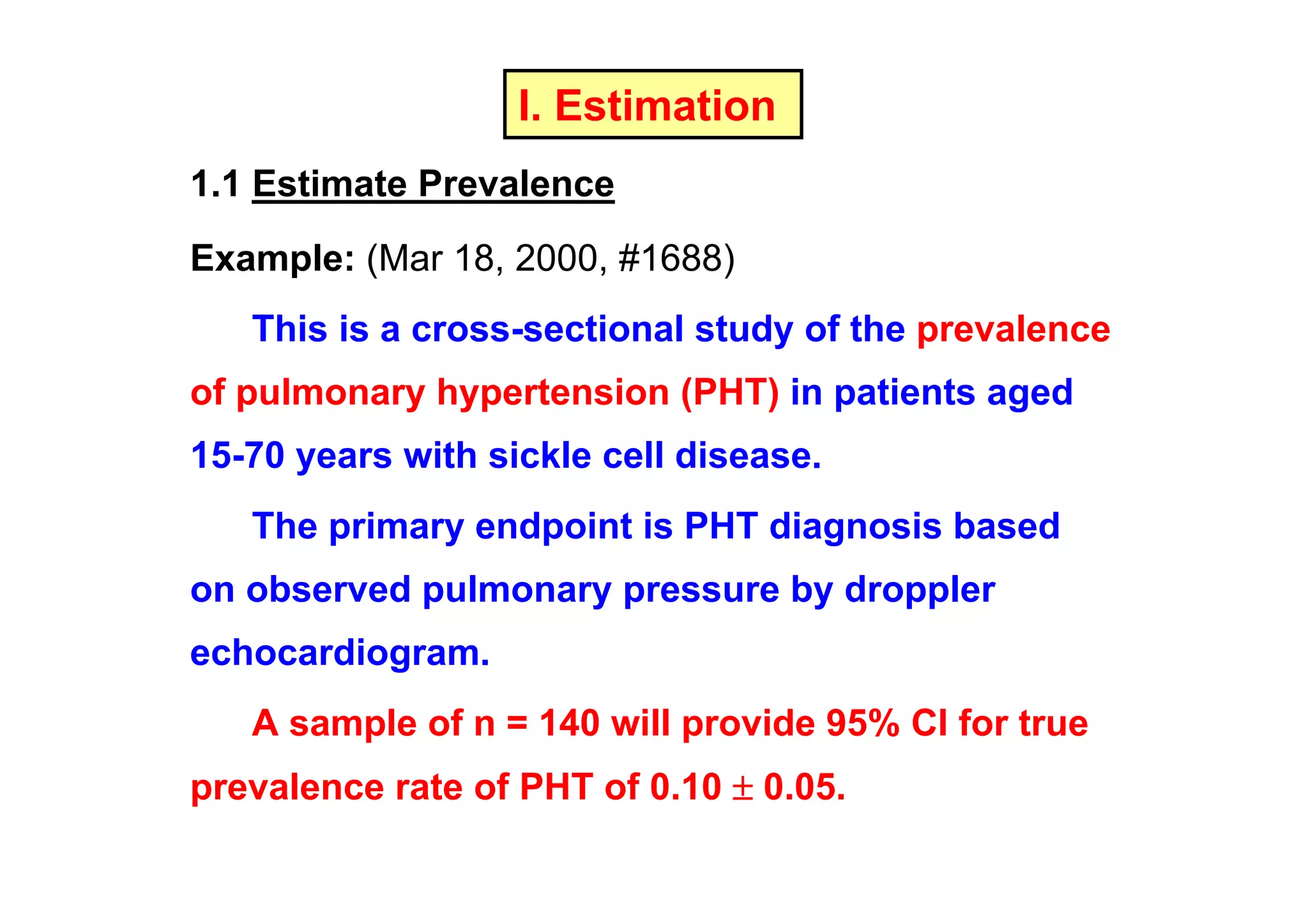
I. Estimation
1.1 Estimate Prevalence
Example: (Mar 18, 2000, #1688)
This is a cross-sectional study of the prevalence
of pulmonary hypertension (PHT) in patients aged
15-70 years with sickle cell disease.
The primary endpoint is PHT diagnosis based
on observed pulmonary pressure by droppler
echocardiogram.
A sample of n = 140 will provide 95% CI for true
prevalence rate of PHT of 0.10 ± 0.05.

95% CI for true prevalence (π) = 0.10 ± 0.05
(1- α)100%
″
= p ± d
= p ± zα/2√pq/n
d = zα/2√pq/n
solve for n
2

zα/2 pq
n =
2
d
where

p = estimated prevalence = 0.1
q = 1-p
= 0.9
d = allowable error in estimating prevalence
(margin of error)
= 0.05
α = probability of type I error
= 0.05 (2-sided), z 0.025 = 1.96

1.96 2 (0.1)(0.9)
n =
= 138.3 = 139
2
0.05

How big is d ?
1. Absolute d
2. Relative d: d ≤ 20% of prevalence(p)
p

d

95% CI

n

0.80

0.05*p = 0.04
0.05
0.10*p = 0.08
0.10
0.15*p = 0.12
0.15
0.20*p = 0.16
0.20

0.76, 0.84
0.75, 0.85
0.72, 0.88
0.70, 0.90
0.68, 0.92
0.65, 0.95
0.64, 0.96
0.60, 1.00

384
246
96
62
43
28
24
16

2

zα/2 pq
n =
2
d

pq
d (error)
α

n

I. Estimation (cont’d)
1.2 Estimate Sensitivity, Specificity
Example:
- 95% CI for Sensitivity = 85% ± 5%
- 95% CI for Specificity = 90% ± 5%

nDi
=?
nNon-Di = ?

Gold standard
+
Test +
a
b
c
d
a+c
b+d
Sensitivity = a / (a+c)
Specificity = d / (b+d)

Sensitivity
Specificity

p±d
85 ± 5
90 ± 5

95% CI
(80, 90)
(85, 95)

n
= 196
nDi
nNon-Di = 139

Ex.
Title: Diagnosis of Benign Paraxysmal Positional Vertigo (BPPV)
by Side-lying test as an alternative to the Dix-Hallpike test
Investigator: Dr. Saowaros Asawavichianginda
Design:

Diagnostic study

Subjects:

Dizzy patients, aged 18-80 yrs, onset < 2 wks

Dizzy pts.
1. Dix-Hallpike test
2. Side-lying test

BPPV

No BPPV

Sample size: Based on 95% CI of true sensitivity (Sn) = 0.9 ± 0.1
2

zα/2 pq
n =
2
d
where

p
q
d
α

=
=
=
=

expected sensitivity = 0.9
1-p = 0.1
allowable error = 0.1
0.05 (2-sided), Z0.025 = 1.96

So, n = 34.56 = No. of patients with BPPV from Dix-Hallpike test
Since prevalence of BPPV among dizzy patients = 40%
Thus, no. of dizzy patients = 34.56 = 86.4 = 87
0.4
Dix-Hallpike test (Gold std)
+ (BPPV)
- (No BPPV)
Side-lying test

+

Sn

-

1 – Sn
35

52

87

1.3 Estimation of 1 Mean

การศึกษานี้มีวัตถุประสงคเพื่อประมาณคาเฉลี่ยของ subcarinal angle
ในคนไทยปกติ และจากการศึกษาของ ... ในคนปกติจํานวน 100 รายอายุ ... ป
พบวาคาเฉลี่ยของ subcarinal angle เทากับ 60.8 (SD=11.8)
ถากําหนดให 95% confidence interval (CI) ของคาเฉลี่ยของ
subcarinal angle ในประชากรไทย (μ) มีคาเทากับ 61 ± 2 (SD=13)
จะตองทําการศึกษาในคนไทยปกติจํานวน 163 คนดังรายละเอียดการคํานวณดังนี้
เมื่อ

ดังนั้น

n = [zα/2 SD / d]2
SD = Standard deviation ของ subcarinal angle
= 13
d = Margin of error ในการประมาณคาเฉลี่ย = 2
α = Probability of type I error (2-sided) = 0.05
z0.025 = 1.96
n = [1.96*13/2]2 = 162.31 = 163

II. Test
2.1 Test for Difference in 2 Independent Proportions
Example: (May 25, 1999, #1549)
This is a randomized (1:1), double-blind,
parallel-group, multi-center trial of drug A (dose1, 2)
in chronic hepatitis C patients aged 18+ years.
The primary efficacy endpoint is sustained viral
response rate after treatment.
N = 141 per group will provide 80% power to detect
an absolute difference in sustained viral response rate
of 11% (7% vs. 18%) at 2-sided α of 0.05.

Clinical significance vs. Statistical significance
an absolute difference in sustained viral response rate
of 11% (7% vs. 18%) at 2-sided α of 0.05.

Clinical (Practical) significance
Statistical significance

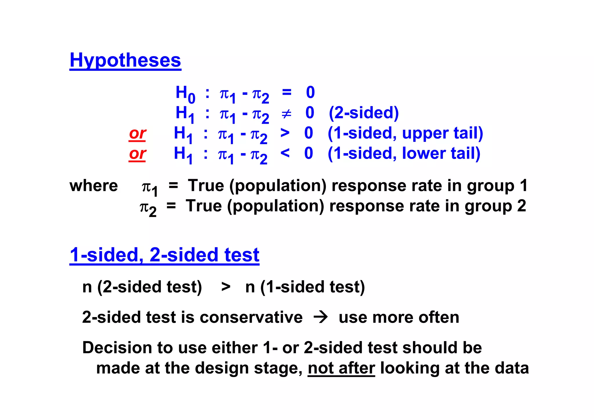
Hypotheses

or
or
where

H0
H1
H1
H1

:
:
:
:

π1 - π2
π1 - π2
π1 - π2
π1 - π2

=
≠
>
<

0
0 (2-sided)
0 (1-sided, upper tail)
0 (1-sided, lower tail)

π1 = True (population) response rate in group 1
π2 = True (population) response rate in group 2

1-sided, 2-sided test
n (2-sided test)

> n (1-sided test)

2-sided test is conservative

use more often

Decision to use either 1- or 2-sided test should be
made at the design stage, not after looking at the data

α, β (Efficacy trial)
Truth
H0 true
(A=B)
Decision
(from p-value)

Accept H0

Reject H0

No error (1- α)
α

H0 false
(A≠B, Difference)
β
No error (1- β)
Power

α

= Pr (incorrect conclusion of difference
= False positive (FP)

β

=
=
=
=

1-β

)

Pr (incorrect conclusion of equivalence)
False negative (FN)
Pr ( correct conclusion of difference )
True positive (TP)

Truth
H0 true
(Not guilty)
Decision Accept H0
(Not guilty)
Reject H0
(Guilty)

H0 false
(Guilty)

No error, 1-α

Type II error, β

Type I error, α

No error, 1-β,
Power

α = Probability of wrongly put innocent person into jail
β = Probability of wrongly set the criminal free
1-β = Probability of correctly put criminal into jail
α is more important than β, so usually set β = 4 α

How big is α, β?
1. Type I error (α, test size, significance level)
- To replace a standard drug with a new drug,
type I error is serious,
use small α (0.01, 0.02)
- To add to the body of the published knowledge,
type I error is less serious
use α = 0.05, 0.10

2. Type II error (β)

- Power (1 - β)
- Power is conventionally set at 80% - 90%
- Typically, α is 4 times as serious as β
α = 0.05, β = 0.20 (power = 0.80)

Calculation: n1 = n2 = n
Based on Chi-square test without continuity correction
Zα if 1-sided

n/group = [
where

zα/2 2pq + z β p1q1 + p 2 q 2
p1 − p 2

]2

p1 = response rate in group 1 = 0.07
= 0.93
q1 = 1 - p1
p2 = response rate in group 2 = 0.18
q2 = 1 – p2
= 0.82
p
q

= (p1 + p2) / 2
= 1–p

α = 0.05 (2-sided),
1- β = 0.80,
n/group = 141

= 0.125
= 0.875
z0.025 = 1.96
z0.2
= 0.842

n / group
α = 0.05
2-sided 1-sided

p1

p2

Power

7

18

80
90

141
188

111
153

7

20

80
90

108
144

85
117

(p1 – p2)
Power
α

n

Based on Chi-square test with continuity correction

n′ =

n
4

⎤
⎡
4
⎥
⎢1 + 1 +
n p1 - p 2 ⎥
⎢
⎦
⎣

2

141 ⎡
4
=
⎢1 + 1 +
4 ⎢
141 0.18 - 0.07
⎣
= 158.7 ~ 159

⎤
⎥
⎥
⎦

2

Ex:
Title: Efficacy of polyethylene plastic wrap for the prevention of
hypothermia during the immediate postnatal period in low
birth weight premature infants
Investigator: Dr. Santi Punnahitananda
Design:

RCT, 2-parallel arms

Subjects: Infants with ≤ 34 gestational wks, birth weight ≤ 1800 gms

Outcome: Infant’s body temperature taken on nursery admission
Infants, ≤ 34 gestational wks, BW ≤ 1800 gms
Randomization

Plastic wrap

No Plastic wrap

Body temp.
Hypothermia

Body temp.
Hypothermia

Sample size estimation: Based on Test of 2 independent proportions
Our unit

hypothermia in low birth weight, premature infants = 55%
(p1 = 0.55)

Assume that plastic wrap would reduce hypothermia to 20%
(p2 = 0.2)

n/group = [

zα/2 2pq + z β p1q1 + p 2 q 2
p1 − p 2

]

2

ตัวอยาง
ในการศึกษาเพื่อหาปจจัยตางๆที่มีความสัมพันธกับการพยายามทํารายตนเอง
ผูวิจัยสนใจในผลของการมีประวัติการเจ็บปวยดวยโรคทางจิตตอการพยายามทํา
รายตนเอง
การศึกษาในอดีตพบวาผูปวยที่ไมเคยทํารายตนเอง (control) มีประวัติการ
เจ็บปวยดวยโรคทางจิต 4% และผูวิจัยคาดวาผูปวยที่เคยทํารายตนเองแตไม
เสียชีวิต (case) จะมีประวัติการเจ็บปวยดวยโรคทางจิตมากกวาคือ 10%
เนื่องจากโดยปกติจํานวนผูปวยที่ไมเคยทํารายตนเองมีมากกวาจํานวนผูปวยที่
เคยทํารายตนเอง จึงกําหนดให control มีจํานวนเปน 2 เทาของ case
เพื่อใหการศึกษานี้มี power 80% ในการพบวาความแตกตางของประวัติการ
เจ็บปวยดวยโรคทางจิต 10% vs. 4% มีนัยสําคัญทางสถิติที่ 2-sided type
I error = 0.05 จะตองใช case 200 คนและ control 400 คน

n1 = ncase = [zα/2√(r+1)pq + zβ√r p1q1 + p2q2 ]2
r (p1 – p2)2

เมื่อ

r = n2/n1 = ncontrol / ncase = 2
ิ

p1 = สัดสวนการมีประวัตการเจ็บปวยดวยโรคทางจิตในกลุม case = 0.10
q1 = 1- p1 = 0.90

ิ

p2 = สัดสวนการมีประวัตการเจ็บปวยดวยโรคทางจิตในกลุม control = 0.04
q2 = 1- p2 = 0.96

p = (p1 + rp2) / (r+1) = 0.06
q = 1- p = 0.94
α =
β =

ดังนั้น

โอกาสที่จะเกิด type I error = 0.05 (2-sided), z0.025 = 1.96
โอกาสที่จะเกิด type II error = 0.2, z0.2 = 0.842
ncase

=

[0.8062 + 0.3935]2 = 199.9
0.0072

II. Test (cont’d)
2.2 Test for Difference of 2 Independent Means
Example: (Aug 24, 1999, #1575)
For patients with idiopathic membranous
glomerulopathy, a phase II, randomized (1:1),
double-blind, placebo-controlled, multi-center
study of drug A will be conducted to determine efficacy.
The primary efficacy endpoint is the change from
baseline in proteinuria at Week 18.
a difference in mean change in loge of urine protein of
–1.22 for placebo and –2.00 for an active drug,
assuming SD = 1.30, 2-sided α of 0.05.
A drop-out rate of 20% is expected, so N = 55 per group
will be recruited.

id

trt

1
2

0
0

n1

0

n1+1
n1+2

1
1

n1+n2

ln_pro0

ln_pro18

pro_d

1

trt: 0=placebo, 1=Drug A
ln_pro0 = loge of proteinurea at Wk 0 (baseline)
ln_pro18 = loge of proteinurea at Wk 18
pro_d
= change at Wk18 of loge of proteinurea from baseline

Hypotheses

or
or

H0
H1
H1
H1

:
:
:
:

μ1 - μ2
μ1 - μ2
μ1 - μ2
μ1 - μ2

=
≠
>
<

0
0 (2-sided)
0 (1-sided, upper tail)
0 (1-sided, lower tail)

where μ1 = true (population) mean in group 1
μ2 = true (population) mean in group 2

Zα if 1-sided


n/group = 2 [

(zα/2 + z β )σ
Δ

]

2

σ = Common standard deviation of change in
loge urine protein
= 1.30
(σ1 = σ2 = σ)
Δ = Difference in mean change between 2 groups
that is considered clinically important
= (-1.22) – (-2.00)
= 0.78
Δ / σ = Effect size (ES)
= effect of treatment in SD unit
α = 0.05 (2-sided), z0.025 = 1.96
z0.2
= 0.842
1 - β = 0.80,

where

Drop-out 20%

n / group =
n / group =

44
44
= 55
(1- dropout)

Δ

σ

0.78

Power

n / group
45
60

80

60

1.30

80

108

1.50

n/group = 2 [

80
90

1.50
0.50

1.30

80

143

(zα/2 + z β )σ
Δ

]2

(mean1 – mean2)
σ
Power
α

n

Ex:
Title: Can knee immobilization after total knee replacement (TKA)
save blood from wound drainage
Investigator: Dr. Vajara Wilairatana
Design:

Randomized controlled trial

Subjects:

Pts. with hip disease that require TKA

Pts. with hip disease that require TKA
Randomization
Knee elevation 40°

Blood loss

A-P splint and
Knee elevation 40°
Blood loss

n/group = 2 [

(zα/2 + z β )σ
Δ

]

2

where
Δ = Difference in mean postoperative blood loss
between 2 groups
σ = SD of postoperative blood loss
Kim YH et al.
Knee splint in 69 knees, mean wound drainage = 436 ml,
SD = 210 ml
Ishii et al.
30 non-splint knees, mean blood loss = 600 ml, SD = 293

Ex:
Title: Early postoperative pain and urinary retention after closed
hemorrhoidectomy: Comparison between spinal and
local anesthesia
Investigator: Dr. Sahapol Anannamcharoen
Design:

RCT

Subjects:

Pts. with grade 3 or 4 hemorrhoidal disease

Pts. with hemorrhoidal disease
Randomization
Spinal anesthesia

Perianal nerve block

Visual analogue scale (VAS) pain score (0-10)

Sample size if parametric test (2-sample t-test) is used

Sample size if Non-parametric (Mann-Whitney) test is used
(VAS pain score is usually positively skewed !!)

II. Test
2.4 Test of Significance of 1 Proportion
Example: (Feb 29, 2000, #1649)
N = 100 subjects with nontuberculous mycobacteria
infection will be recruited for this multi-center study.
The primary objective is to test if the frequency of
cystic fibrosis transmembrane conductance regulator
(CFTR) gene mutation is 4%. If more CF carriers are
found at a statistically significant number, then this
would suggest that CFTR alleles may be important in
predisposing to this disease.
N = 96 will provide 90% power to test H0 : π = π0 = 0.04,
against 1-sided H1 : π = π1 = 0.115, using α = 0.05.

Hypotheses
H0 : π = π0 (π0 = 0.04 )
H1 : π > π0 (π1 = 0.115)

Calculation

n =[
where

zα p 0 q 0 + z β p1q1
p 0 − p1

p0 =
q0 = 1 – p0

0.04
= 0.96

p1 =
q1 = 1 – p1

]

2

0.115
= 0.885

α = 0.05 (1-sided), z0.05 = 1.645
1- β = 0.90,
z0.1 = 1.282
n = 96

II. Test (cont’d)
2.5 Test of Significance of 1 Mean
Example:
The average weight of men over 55 years of age
with newly diagnosed heart disease was 90 kg.
However, it is suspected that the average weight is
now somewhat lower.
How large a sample would be necessary to test,
at 5% level of significance with a power of 90%,
whether the average weight is unchanged versus
the alternative that it has decreased from 90 to 85 kg
with an estimated SD of 20 kg?

Hypotheses
H0 : μ = μ0 (μ0 = 90)
H1 : μ < μ0 (μ1 = 85)

Calculation

n = [
where

(z α + z β )σ
Δ

σ = estimated SD
Δ = | μ1 - μ0|

]

2

= 20
= 5

α = 0.05 (1-sided), z0.05 = 1.645
1- β = 0.90,
z0.1 = 1.282
n = 137.08 = 138

II. Test (cont’d)
2.6 Test of Significance of 1 Correlation Coefficient
H0: ρ = ρ0
H1: ρ = ρ1

“การศึกษาความสัมพันธระหวางการวัดพังผืดในตับดวยวิธี
Transient Elastography กับการวินิจฉัยดวยวิธีเจาะชิ้นเนือตับใน
้
ผูปวยโรคเรื้อนกวาง (psoriasis)ที่ไดรับการรักษาดวยยาเมโธเทร็กเซท
(methotrexate; MTX) ในคนไทย”
จากวัตถุประสงคหลักของการวิจัยเพื่อหาความสัมพันธระหวาง
คาที่ไดจากการวัดพังผืดในตับดวยวิธี Transient Elastography
กับคาที่ไดจากการวินิจฉัยภาวะพังผืดดวยวิธีเจาะชิ้นเนือตับ การ
้
คํานวณขนาดตัวอยางจึงเปนการคํานวณเพื่อทดสอบคา Correlation
coefficient โดยมีสมมติฐานทางสถิติดงนี้
ั
H0 : ρ 0 = 0
H1 : ρ1 = 0.3 (Ref #1)

n

=

(Zα/2 + Zβ)

2

+ 3

[F(Z0) + F(Z1)]
α = Probability of type I error = 0.05 (2-sided)
Z0.025 = 1.96
β = Probability of type II error = 0.1
1-β = Power = 0.90
Z0.1 = 1.282
F(Z)

= Fisher’s Z transformation
= 0.5 ln [(1+ρ)/(1-ρ)]

Under H0: ρ=0

F(Z0) = 0.5 x ln [(1+0)/(1-0)]

Under H1: ρ=0.3

F(Z1) = 0.5 x ln [(1+0.3)/(1-0.3)] = 0.31

Thus,
n = [ (1.96+1.282)/(0-0.31) ]2 + 3
= 112.4 = 113

= 0

More than one primary outcome
If one of these endpoints is regarded as more important
than others, then calculate n for that primary endpoint.
If several outcomes are regarded as equally important,
then calculate n for each outcome in turn,
and select the largest n as the sample size required to
answer all the questions of interest.

Caution:
Calculation of sample size needs a number of
assumptions and ‘guesstimates’,
so such calculation only provides a guide to the
number of subjects required.

Sample size estimation:
1. Formulas
2. Published tables, nomograms
3. Softwares e.g.,
- nQuery Advisor
- PS (Power and Sample Size Program)
- etc.

References
Blackwelder WC. Proving the Null Hypothesis in Clinical
Trials. Controlled Clinical Trials 1982; 3: 345-353.
Breslow NE, Day NE. Statistical Methods in Cancer
Research Vol. II – The Design and Analysis of Cohort
Studies. Oxford : Oxford University Press; 1987.
Chow SC, Liu JP. Design and Analysis of Clinical Trials.
Concept and Methodologies. New York: John Wiley & Sons,
Inc. 1998.
Fleiss JL. Statistical Methods for Rates and Proportions.
New York : John Wiley & Sons; 1981.
Karlberg J, Tsang K. Introduction to Clinical Trials: Clinical
Trials Research Methodology, Statistical Methods in Clinical
Trials, The ICH GCP Guidelines. Hong Kong: The Clinical
Trials Centre. 1998.

Lachin JM. Introduction to Sample Size Determination
and Power Analysis for Clinical Trials. Controlled Clinical
Trials 1981; 2: 93-113.
Lemeshow S, Hosmer DW, Klar J, Lwanga SK.
Adequacy of Sample Size in Health Studies. New York :
John Wiley & Sons; 1990.

Sample size estimation

In this document

More Related Content

What's hot

Similar to Sample size estimation

Recently uploaded

Sample size estimation