This document discusses seismic velocities and how they are affected by rock properties. It contains the following key points:
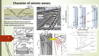
1. Seismic waves can be classified as body waves, which travel through rock, and surface waves, which travel along surfaces. Body waves are P waves and S waves, with P waves traveling faster.
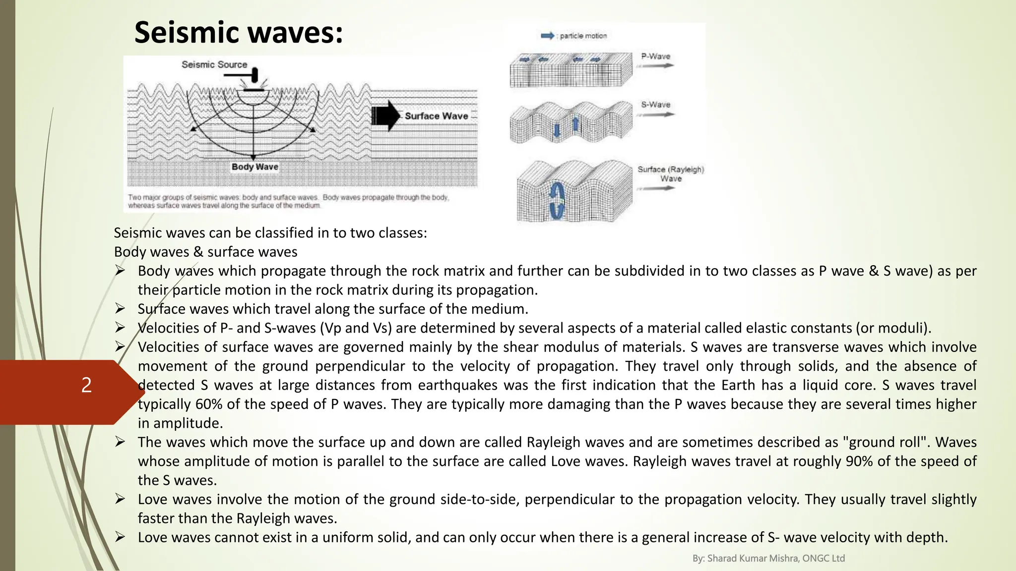
2. The velocities of P and S waves are determined by elastic properties of the material like density, bulk modulus, and shear modulus. S wave velocity is always lower than P wave velocity.
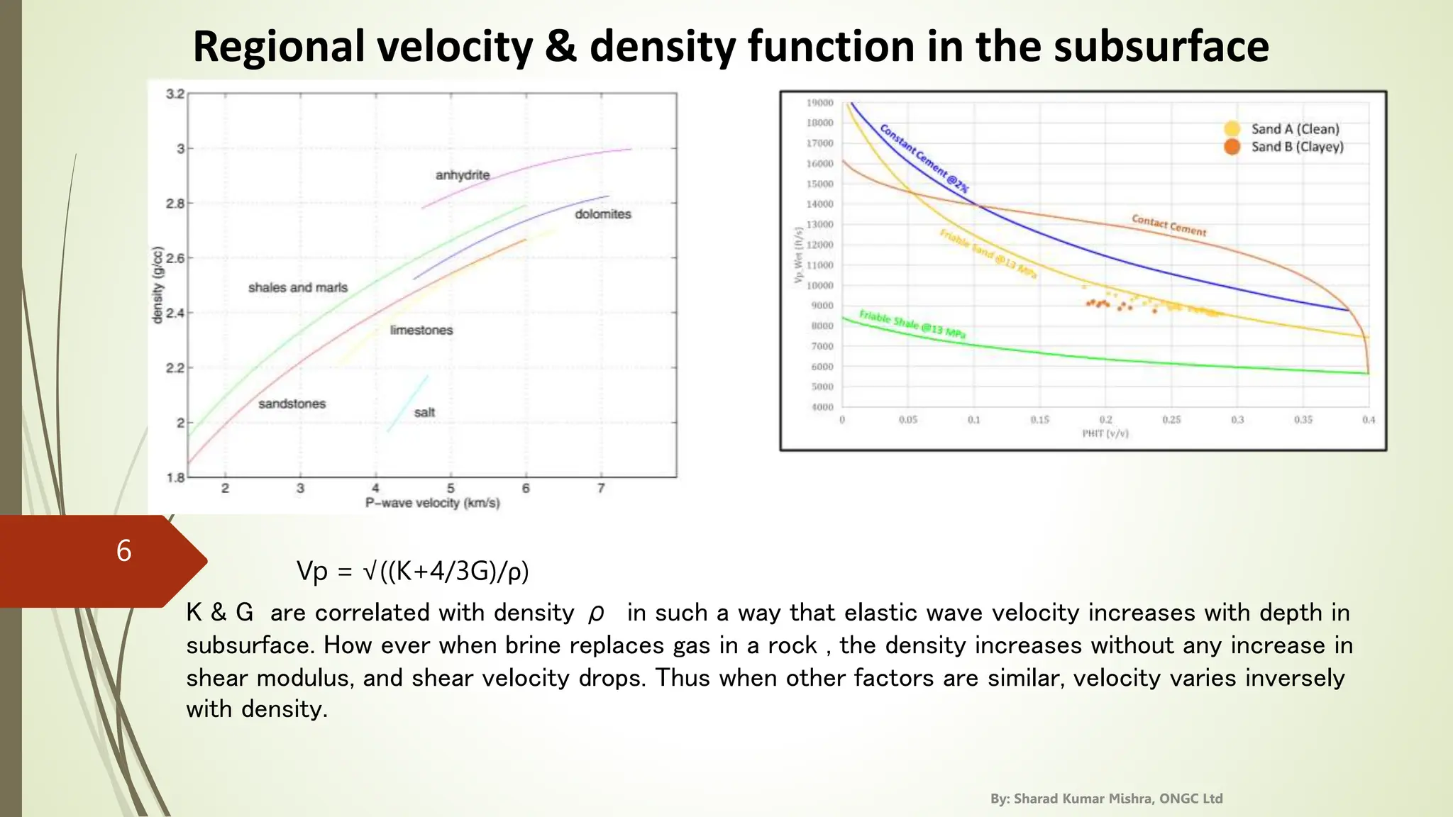
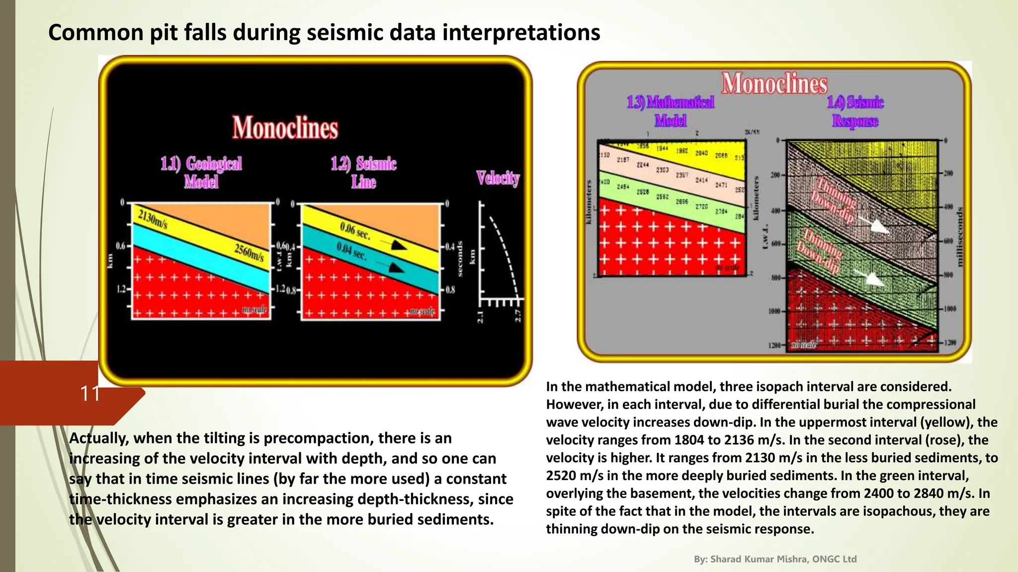
3. Seismic velocities increase with depth and density in the subsurface generally, though velocity can decrease if gas is replaced by brine in rocks. Lateral velocity changes can cause seismic artifacts like pull up